Nave Bayes and Hadoop Shannon Quinn http xkcd

Naïve Bayes and Hadoop Shannon Quinn

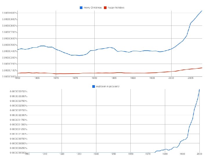
http: //xkcd. com/ngram-charts/

Coupled Temporal Scoping of Relational Facts. P. P. Talukdar, D. T. Wijaya and T. M. Mitchell. In Proceedings of the ACM International Conference on Web Search and Data Mining (WSDM), 2012 Understanding Semantic Change of Words Over Centuries. D. T. Wijaya and R. Yeniterzi. In Workshop on Detecting and Exploiting Cultural Diversity on the Social Web (DETECT), 2011 at CIKM 2011

Some of A Joint Distribution A B C D E is the effect of the 0. 00036 is the effect of a 0. 00034 . The effect of this 0. 00034 to this effect : “ 0. 00034 be the effect of the … … … the effect of any 0. 00024 … … … does not affect the general 0. 00020 does not affect the question 0. 00020 any manner affect the principle 0. 00018 not p
 avg of 1. 5 examples per")
Flashback Size of table: 215=32768 (if all binary) avg of 1. 5 examples per row Actual m = 1, 974, 927, 360 (if continuous attributes binarized) Abstract: Predict whether income exceeds $50 K/yr based on census data. Also known as "Census Income" dataset. [Kohavi, 1996] Number of Instances: 48, 842 Number of Attributes: 14 (in UCI’s copy of dataset) + 1; 3 (here)

Naïve Density Estimation The problem with the Joint Estimator is that it just mirrors the training data (and is *hard* to compute). We need something which generalizes more usefully. The naïve model generalizes strongly: Assume that each attribute is distributed independently of any of the other attributes. Copyright © Andrew W. Moore

Using the Naïve Distribution • Once you have a Naïve Distribution you can easily compute any row of the joint distribution. • Suppose A, B, C and D are independently distributed. What is P(A ^ ~B ^ C ^ ~D)? Copyright © Andrew W. Moore

Using the Naïve Distribution • Once you have a Naïve Distribution you can easily compute any row of the joint distribution. • Suppose A, B, C and D are independently distributed. What is P(A ^ ~B ^ C ^ ~D)? P(A) P(~B) P(C) P(~D) Copyright © Andrew W. Moore

Naïve Distribution General Case • Suppose X 1, X 2, …, Xd are independently distributed. • So if we have a Naïve Distribution we can construct any row of the implied Joint Distribution on demand. • How do we learn this? Copyright © Andrew W. Moore
 Another trivial learning algorithm! Copyright ©")
Learning a Naïve Density Estimator MLE Dirichlet (MAP) Another trivial learning algorithm! Copyright © Andrew W. Moore
=Pr(A)Pr(B)")
Independently Distributed Data • Review: A and B are independent if – Pr(A, B)=Pr(A)Pr(B) – Sometimes written: • A and B are conditionally independent given C if Pr(A, B|C)=Pr(A|C)*Pr(B|C) – Written Copyright © Andrew W. Moore
… • … in")
Bayes Classifiers • If we can do inference over Pr(X, Y)… • … in particular compute Pr(X|Y) and Pr(Y). – We can compute

Can we make this interesting? Yes! • Key ideas: – Pick the class variable Y – Instead of estimating P(X 1, …, Xn, Y) = P(X 1)*…*P(Xn)*Y, estimate P(X 1, …, Xn|Y) = P(X 1|Y)*…*P(Xn|Y) – Or, assume P(Xi|Y)=Pr(Xi|X 1, …, Xi-1, Xi+1, …Xn, Y) – Or, that Xi is conditionally independent of every Xj, j!=i, given Y. – How to estimate? MLE

The Naïve Bayes classifier – v 1 • Dataset: each example has – A unique id id • Why? For debugging the feature extractor – d attributes X 1, …, Xd • Each Xi takes a discrete value in dom(Xi) – One class label Y in dom(Y) • You have a train dataset and a test dataset

The Naïve Bayes classifier – v 1 • You have a train dataset and a test dataset • Initialize an “event counter” (hashtable) C • For each example id, y, x 1, …. , xd in train: – C(“Y=ANY”) ++; C(“Y=y”) ++ – For j in 1. . d: • C(“Y=y ^ Xj=xj”) ++ • For each example id, y, x 1, …. , xd in test: – For each y’ in dom(Y): • Compute Pr(y’, x 1, …. , xd) = – Return the best y’

The Naïve Bayes classifier – v 1 • You have a train dataset and a test dataset • Initialize an “event counter” (hashtable) C • For each example id, y, x 1, …. , xd in train: – C(“Y=ANY”) ++; C(“Y=y”) ++ – For j in 1. . d: • C(“Y=y ^ Xj=xj”) ++ • For each example id, y, x 1, …. , xd in test: – For each y’ in dom(Y): • Compute Pr(y’, x 1, …. , xd) = This will overfit, so … – Return the best y’

The Naïve Bayes classifier – v 1 • You have a train dataset and a test dataset • Initialize an “event counter” (hashtable) C • For each example id, y, x 1, …. , xd in train: – C(“Y=ANY”) ++; C(“Y=y”) ++ – For j in 1. . d: • C(“Y=y ^ Xj=xj”) ++ • For each example id, y, x 1, …. , xd in test: – For each y’ in dom(Y): • Compute Pr(y’, x 1, …. , xd) = – Return the best y’ where: qj = 1/|dom(Xj)| qy = 1/|dom(Y)| m=1 This will underflow, so …

The Naïve Bayes classifier – v 1 • You have a train dataset and a test dataset • Initialize an “event counter” (hashtable) C • For each example id, y, x 1, …. , xd in train: – C(“Y=ANY”) ++; C(“Y=y”) ++ – For j in 1. . d: • C(“Y=y ^ Xj=xj”) ++ • For each example id, y, x 1, …. , xd in test: – For each y’ in dom(Y): • Compute log Pr(y’, x 1, …. , xd) = – Return the best y’ where: qj = 1/|dom(Xj)| qy = 1/|dom(Y)| m=1

The Naïve Bayes classifier – v 2 • For text documents, what features do you use? • One common choice: – X 1 = first word in the document – X 2 = second word in the document – X 3 = third … – X 4 = … –… • But: Pr(X 13=hockey|Y=sports) is probably not that different from Pr(X 11=hockey|Y=sports)…so instead of treating them as different variables, treat them as different copies of the same variable

The Naïve Bayes classifier – v 1 • You have a train dataset and a test dataset • Initialize an “event counter” (hashtable) C • For each example id, y, x 1, …. , xd in train: – C(“Y=ANY”) ++; C(“Y=y”) ++ – For j in 1. . d: • C(“Y=y ^ Xj=xj”) ++ • For each example id, y, x 1, …. , xd in test: – For each y’ in dom(Y): • Compute Pr(y’, x 1, …. , xd) = – Return the best y’

The Naïve Bayes classifier – v 2 • You have a train dataset and a test dataset • Initialize an “event counter” (hashtable) C • For each example id, y, x 1, …. , xd in train: – C(“Y=ANY”) ++; C(“Y=y”) ++ – For j in 1. . d: • C(“Y=y ^ Xj=xj”) ++ • For each example id, y, x 1, …. , xd in test: – For each y’ in dom(Y): • Compute Pr(y’, x 1, …. , xd) = – Return the best y’

The Naïve Bayes classifier – v 2 • You have a train dataset and a test dataset • Initialize an “event counter” (hashtable) C • For each example id, y, x 1, …. , xd in train: – C(“Y=ANY”) ++; C(“Y=y”) ++ – For j in 1. . d: • C(“Y=y ^ X=xj”) ++ • For each example id, y, x 1, …. , xd in test: – For each y’ in dom(Y): • Compute Pr(y’, x 1, …. , xd) = – Return the best y’

The Naïve Bayes classifier – v 2 • You have a train dataset and a test dataset • Initialize an “event counter” (hashtable) C • For each example id, y, x 1, …. , xd in train: – C(“Y=ANY”) ++; C(“Y=y”) ++ – For j in 1. . d: • C(“Y=y ^ X=xj”) ++ • For each example id, y, x 1, …. , xd in test: – For each y’ in dom(Y): • Compute log Pr(y’, x 1, …. , xd) = – Return the best y’ where: qj = 1/|V| qy = 1/|dom(Y)| m=1

Complexity of Naïve Bayes Sequential reads • You have a train dataset and a test dataset • Initialize an “event counter” (hashtable) C • For each example id, y, x 1, …. , xd in train: Complexity: O(n), n=size of train – C(“Y=ANY”) ++; C(“Y=y”) ++ – For j in 1. . d: • C(“Y=y ^ X=xj”) ++ • For each example id, y, x 1, …. , xd in test: – For each y’ in dom(Y): • Compute log Pr(y’, x 1, …. , xd) = – Return the best y’ where: qj = 1/|V| qy = 1/|dom(Y)| m=1 Sequential reads Complexity: O(|dom(Y)|*n’), n’=size of test

Map. Reduce!

Inspiration not Plagiarism • This is not the first lecture ever on Mapreduce • I borrowed from William Cohen, who borrowed from Alona Fyshe, and she borrowed from: • Jimmy Lin • http: //www. umiacs. umd. edu/~jimmylin/cloud-computing/SIGIR-2009/Lin-Map. Reduce-SIGIR 2009. pdf • Google • • http: //code. google. com/edu/submissions/mapreduce-minilecture/listing. html http: //code. google. com/edu/submissions/mapreduce/listing. html • Cloudera • http: //vimeo. com/3584536

Introduction to Map. Reduce • 3 main phases – Map (send each input record to a key) – Sort (put all of one key in the same place) • Handled behind the scenes in Hadoop – Reduce (operate on each key and its set of values) • Terms come from functional programming: – map(lambda x: x. upper(), [”shannon", ”p", ”quinn"]) [’SHANNON', ’P', ’QUINN'] – reduce(lambda x, y: x+""+y, [”shannon", ”p", ”quinn"]) ”shannon-p-quinn”

Map. Reduce overview Map Shuffle/Sort Reduce

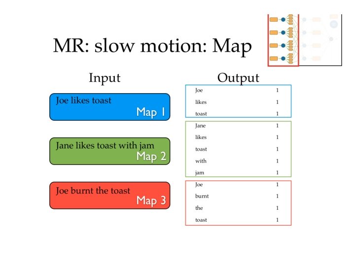
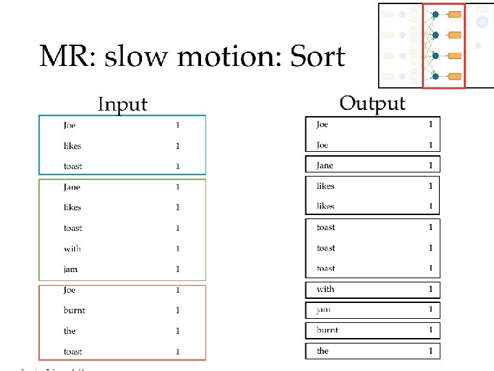
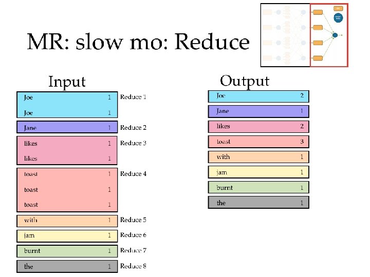
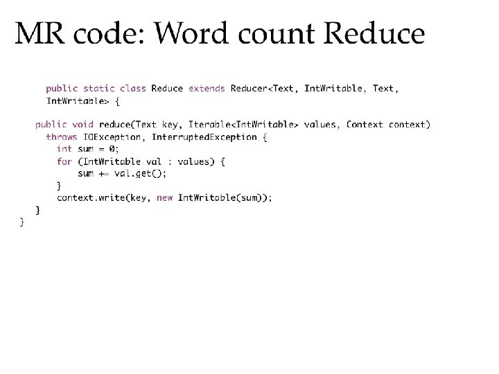
Map. Reduce in slow motion • Canonical example: Word Count • Example corpus:


others: • Key. Value. Input. Format • Sequence. File. Input. Format

Is any part of this wasteful? • Remember - moving data around and writing to/reading from disk are very expensive operations • No reducer can start until: • all mappers are done • data in its partition has been sorted

Common pitfalls • You have no control over the order in which reduces are performed • You have “no” control over the order in which you encounter reduce values – Sort of (more later). • The only ordering you should assume is that Reducers always start after Mappers

Common pitfalls • You should assume your Maps and Reduces will be taking place on different machines with different memory spaces • Don’t make a static variable and assume that other processes can read it – They can’t. – It appear that they can when run locally, but they can’t – No really, don’t do this.

Common pitfalls • Do not communicate between mappers or between reducers – overhead is high – you don’t know which mappers/reducers are actually running at any given point – there’s no easy way to find out what machine they’re running on • because you shouldn’t be looking for them anyway

Assignment 1 • Naïve Bayes on Hadoop • Document classification • Due Thursday, Jan 29 by 11: 59 pm

Other reminders • If you haven’t yet signed up for a student presentation, do so! – I will be assigning slots starting Friday at 5 pm, so sign up before then – You need to be on Bit. Bucket to do this • Mailing list for questions • Office hours Mondays 9 -10: 30 am
- Slides: 48