Natural Language Processing Language Model Language Models Formal

Natural Language Processing Language Model

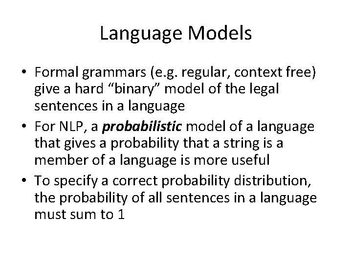
Language Models • Formal grammars (e. g. regular, context free) give a hard “binary” model of the legal sentences in a language • For NLP, a probabilistic model of a language that gives a probability that a string is a member of a language is more useful • To specify a correct probability distribution, the probability of all sentences in a language must sum to 1

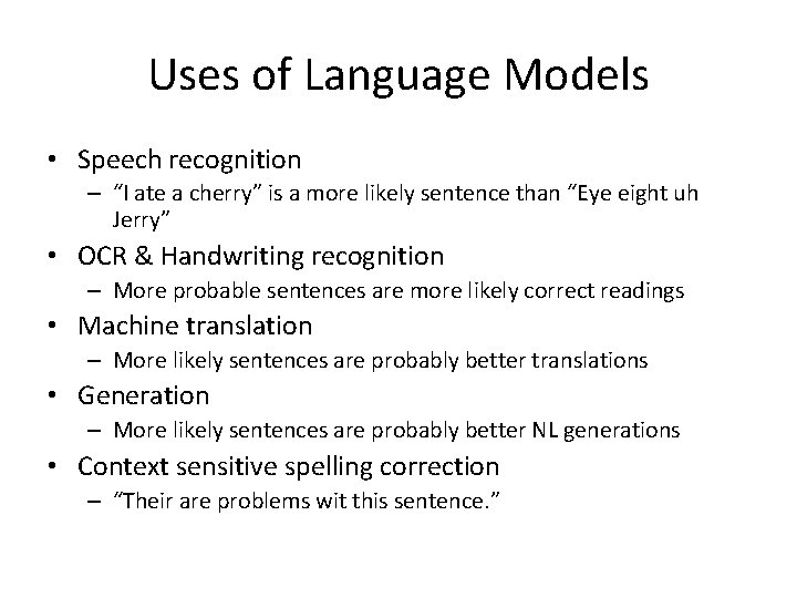
Uses of Language Models • Speech recognition – “I ate a cherry” is a more likely sentence than “Eye eight uh Jerry” • OCR & Handwriting recognition – More probable sentences are more likely correct readings • Machine translation – More likely sentences are probably better translations • Generation – More likely sentences are probably better NL generations • Context sensitive spelling correction – “Their are problems wit this sentence. ”

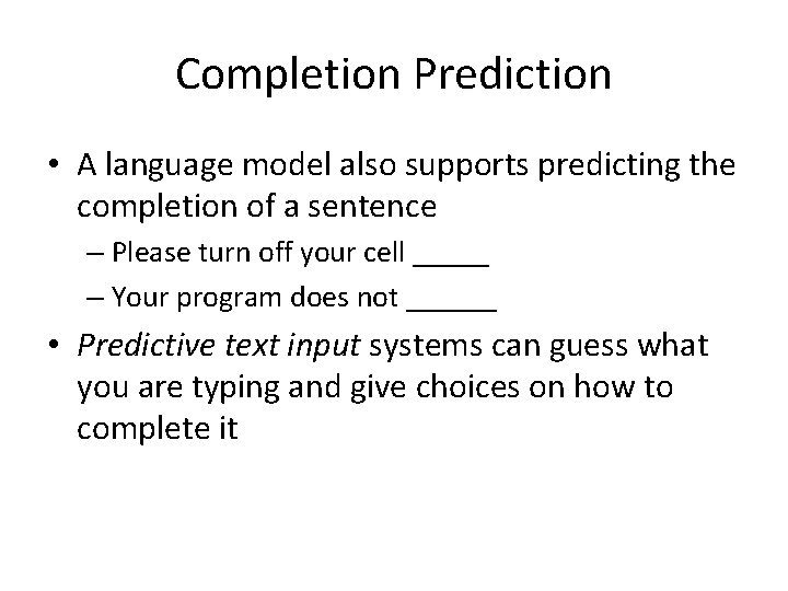
Completion Prediction • A language model also supports predicting the completion of a sentence – Please turn off your cell _____ – Your program does not ______ • Predictive text input systems can guess what you are typing and give choices on how to complete it

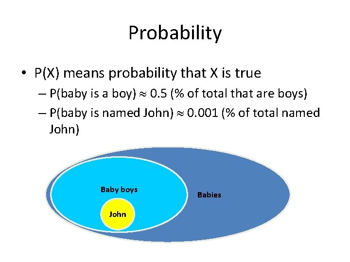
Probability • P(X) means probability that X is true – P(baby is a boy) 0. 5 (% of total that are boys) – P(baby is named John) 0. 001 (% of total named John) Baby boys John Babies

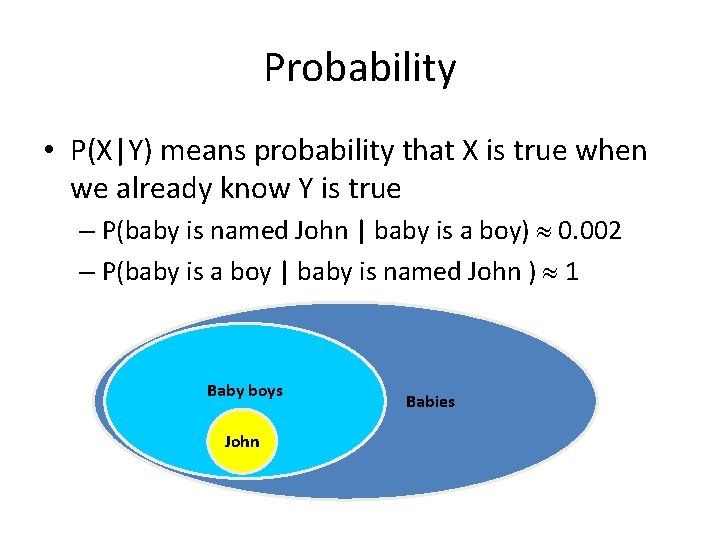
Probability • P(X|Y) means probability that X is true when we already know Y is true – P(baby is named John | baby is a boy) 0. 002 – P(baby is a boy | baby is named John ) 1 Baby boys John Babies

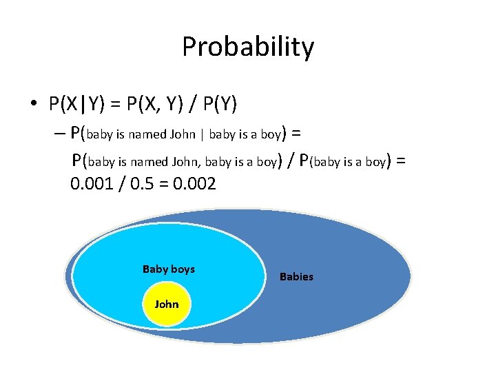
Probability • P(X|Y) = P(X, Y) / P(Y) – P(baby is named John | baby is a boy) = P(baby is named John, baby is a boy) / P(baby is a boy) = 0. 001 / 0. 5 = 0. 002 Baby boys John Babies

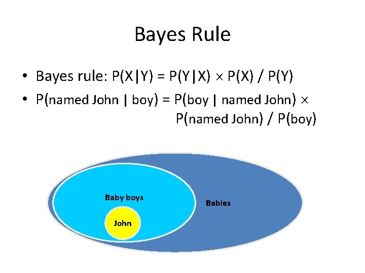
Bayes Rule • Bayes rule: P(X|Y) = P(Y|X) P(X) / P(Y) • P(named John | boy) = P(boy | named John) P(named John) / P(boy) Baby boys John Babies

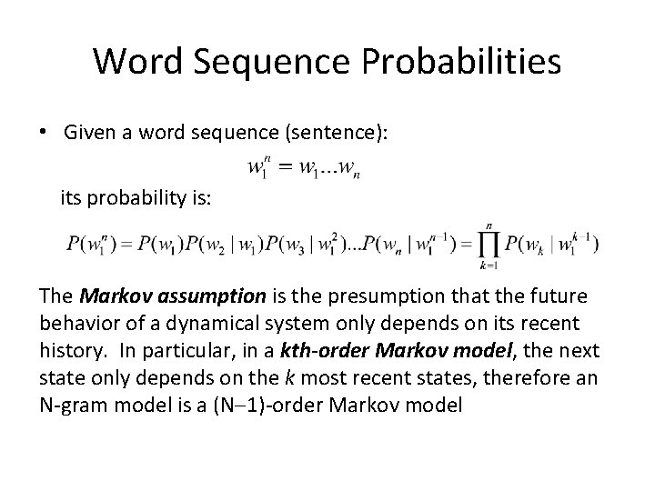
Word Sequence Probabilities • Given a word sequence (sentence): its probability is: The Markov assumption is the presumption that the future behavior of a dynamical system only depends on its recent history. In particular, in a kth-order Markov model, the next state only depends on the k most recent states, therefore an N-gram model is a (N 1)-order Markov model

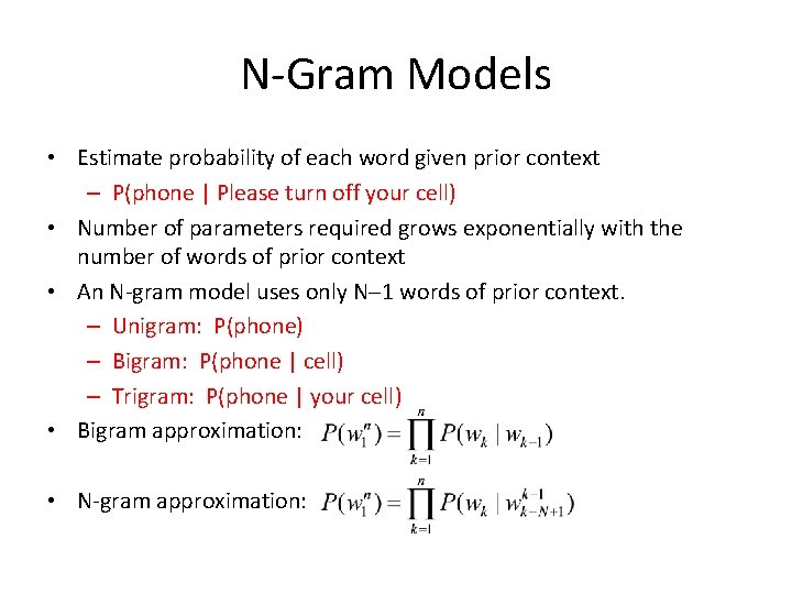
N-Gram Models • Estimate probability of each word given prior context – P(phone | Please turn off your cell) • Number of parameters required grows exponentially with the number of words of prior context • An N-gram model uses only N 1 words of prior context. – Unigram: P(phone) – Bigram: P(phone | cell) – Trigram: P(phone | your cell) • Bigram approximation: • N-gram approximation:

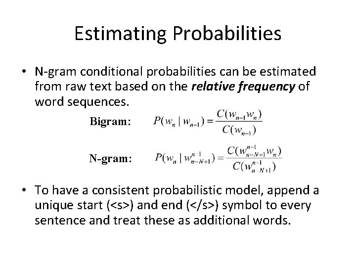
Estimating Probabilities • N-gram conditional probabilities can be estimated from raw text based on the relative frequency of word sequences. Bigram: N-gram: • To have a consistent probabilistic model, append a unique start (<s>) and end (</s>) symbol to every sentence and treat these as additional words.

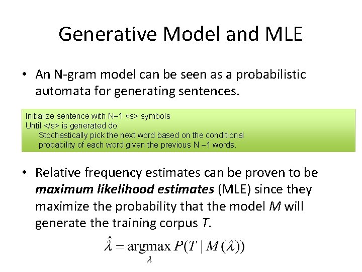
Generative Model and MLE • An N-gram model can be seen as a probabilistic automata for generating sentences. Initialize sentence with N 1 <s> symbols Until </s> is generated do: Stochastically pick the next word based on the conditional probability of each word given the previous N 1 words. • Relative frequency estimates can be proven to be maximum likelihood estimates (MLE) since they maximize the probability that the model M will generate the training corpus T.

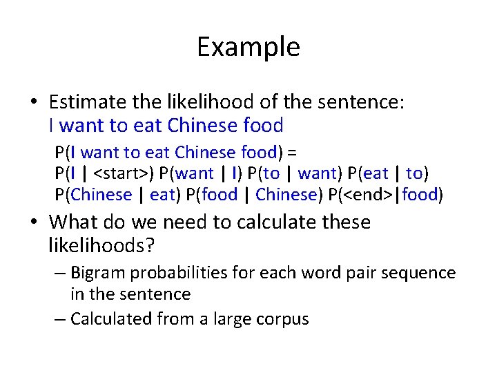
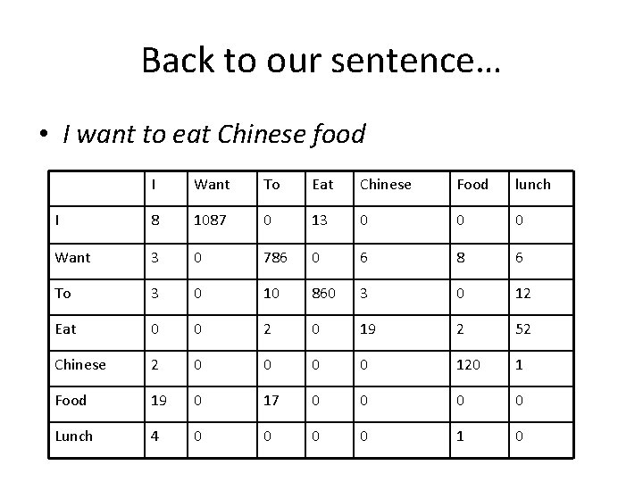
Example • Estimate the likelihood of the sentence: I want to eat Chinese food P(I want to eat Chinese food) = P(I | <start>) P(want | I) P(to | want) P(eat | to) P(Chinese | eat) P(food | Chinese) P(<end>|food) • What do we need to calculate these likelihoods? – Bigram probabilities for each word pair sequence in the sentence – Calculated from a large corpus

Corpus • A language model must be trained on a large corpus of text to estimate good parameter values • Model can be evaluated based on its ability to predict a high probability for a disjoint (held-out) test corpus (testing on the training corpus would give an optimistically biased estimate) • Ideally, the training (and test) corpus should be representative of the actual application data

Terminology • Types: number of distinct words in a corpus (vocabulary size) • Tokens: total number of words

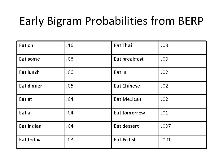
Early Bigram Probabilities from BERP Eat on . 16 Eat Thai . 03 Eat some . 06 Eat breakfast . 03 Eat lunch . 06 Eat in . 02 Eat dinner . 05 Eat Chinese . 02 Eat at . 04 Eat Mexican . 02 Eat a . 04 Eat tomorrow . 01 Eat Indian . 04 Eat dessert . 007 Eat today . 03 Eat British . 001

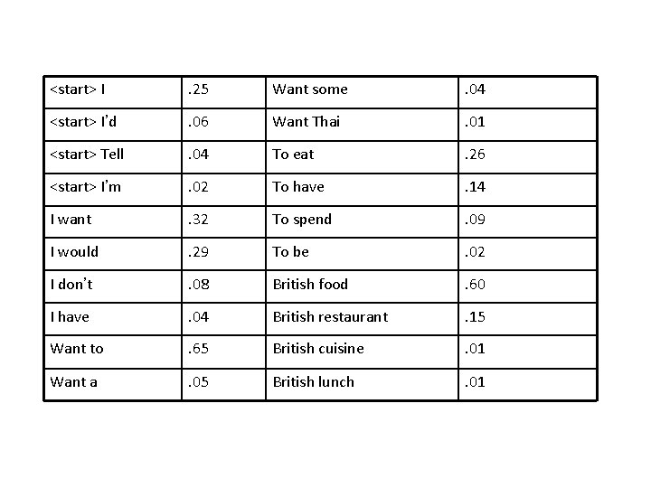
<start> I . 25 Want some . 04 <start> I’d . 06 Want Thai . 01 <start> Tell . 04 To eat . 26 <start> I’m . 02 To have . 14 I want . 32 To spend . 09 I would . 29 To be . 02 I don’t . 08 British food . 60 I have . 04 British restaurant . 15 Want to . 65 British cuisine . 01 Want a . 05 British lunch . 01

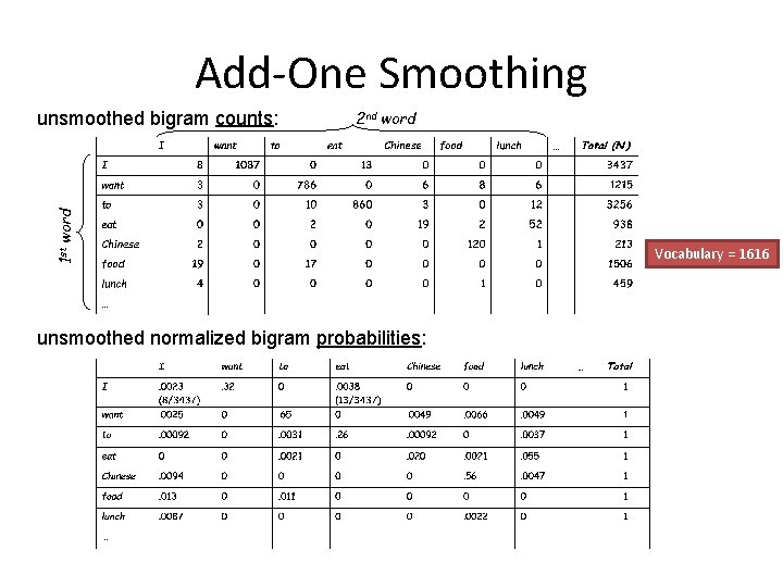
Back to our sentence… • I want to eat Chinese food I Want To Eat Chinese Food lunch I 8 1087 0 13 0 0 0 Want 3 0 786 0 6 8 6 To 3 0 10 860 3 0 12 Eat 0 0 2 0 19 2 52 Chinese 2 0 0 120 1 Food 19 0 17 0 0 Lunch 4 0 0 1 0

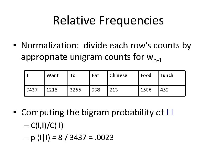
Relative Frequencies • Normalization: divide each row's counts by appropriate unigram counts for wn-1 I Want To Eat Chinese Food Lunch 3437 1215 3256 938 213 1506 459 • Computing the bigram probability of I I – C(I, I)/C( I) – p (I|I) = 8 / 3437 =. 0023

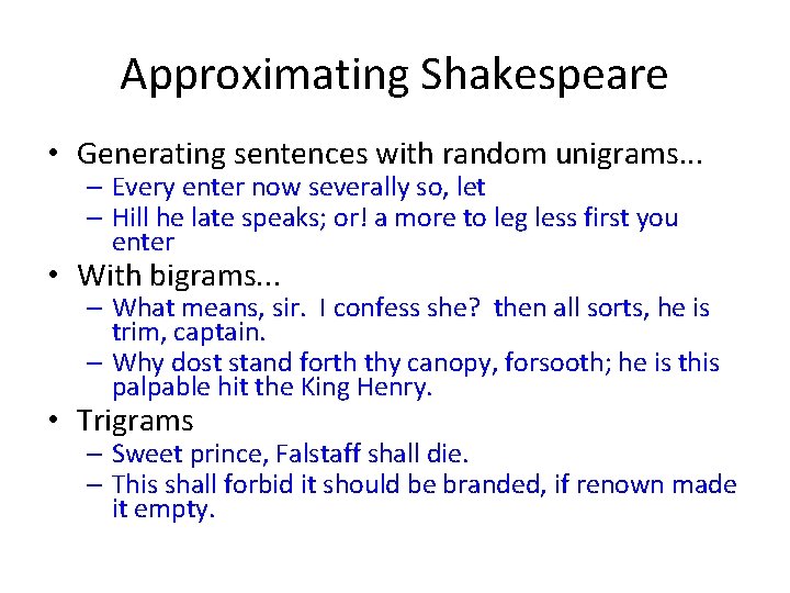
Approximating Shakespeare • Generating sentences with random unigrams. . . – Every enter now severally so, let – Hill he late speaks; or! a more to leg less first you enter • With bigrams. . . – What means, sir. I confess she? then all sorts, he is trim, captain. – Why dost stand forth thy canopy, forsooth; he is this palpable hit the King Henry. • Trigrams – Sweet prince, Falstaff shall die. – This shall forbid it should be branded, if renown made it empty.

Approximating Shakespeare • Quadrigrams – What! I will go seek the traitor Gloucester. – Will you not tell me who I am? – What's coming out here looks like Shakespeare because it is Shakespeare • Note: As we increase the value of N, the accuracy of an n-gram model increases, since choice of next word becomes increasingly constrained

Evaluation • Perplexity and entropy: how do you estimate how well your language model fits a corpus once you’re done?

Random Variables • A variable defined by the probabilities of each possible value in the population • Discrete Random Variable – Whole Number (0, 1, 2, 3 etc. ) – Countable, Finite Number of Values • Jump from one value to the next and cannot take any values in between • Continuous Random Variables – Whole or Fractional Number – Obtained by Measuring – Infinite Number of Values in Interval • Too Many to List Like Discrete Variable

Discrete Random Variables • For example: # of girls in the family # of of correct answers of a given exam …

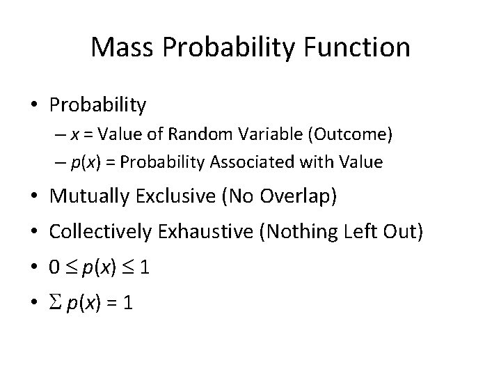
Mass Probability Function • Probability – x = Value of Random Variable (Outcome) – p(x) = Probability Associated with Value • Mutually Exclusive (No Overlap) • Collectively Exhaustive (Nothing Left Out) • 0 p(x) 1 • p(x) = 1

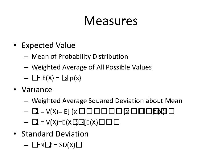
Measures • Expected Value – Mean of Probability Distribution – Weighted Average of All Possible Values – �= E(X) = �x p(x) • Variance – Weighted Average Squared Deviation about Mean – � 2 = V(X)= E[ (x ������ p(x) – � 2 = V(X)=E(X�)�-[E(X)��� • Standard Deviation – �= � 2 = SD(X)�

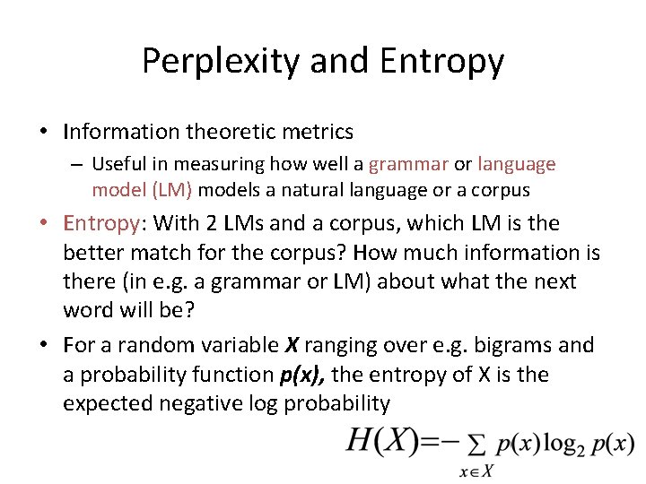
Perplexity and Entropy • Information theoretic metrics – Useful in measuring how well a grammar or language model (LM) models a natural language or a corpus • Entropy: With 2 LMs and a corpus, which LM is the better match for the corpus? How much information is there (in e. g. a grammar or LM) about what the next word will be? • For a random variable X ranging over e. g. bigrams and a probability function p(x), the entropy of X is the expected negative log probability

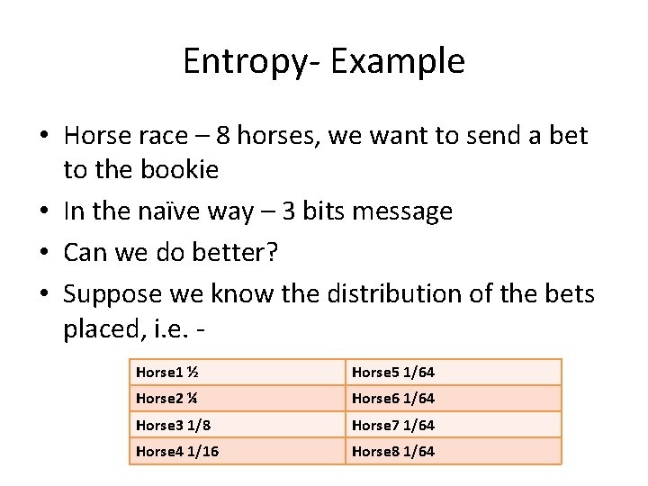
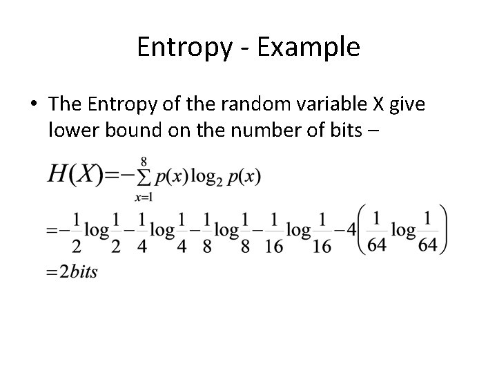
Entropy- Example • Horse race – 8 horses, we want to send a bet to the bookie • In the naïve way – 3 bits message • Can we do better? • Suppose we know the distribution of the bets placed, i. e. Horse 1 ½ Horse 5 1/64 Horse 2 ¼ Horse 6 1/64 Horse 3 1/8 Horse 7 1/64 Horse 4 1/16 Horse 8 1/64

Entropy - Example • The Entropy of the random variable X give lower bound on the number of bits –

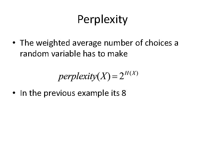
Perplexity • The weighted average number of choices a random variable has to make • In the previous example its 8

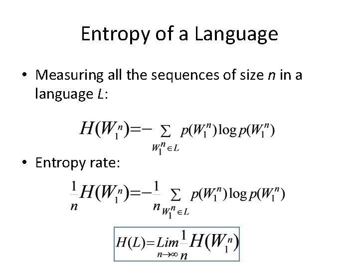
Entropy of a Language • Measuring all the sequences of size n in a language L: • Entropy rate:

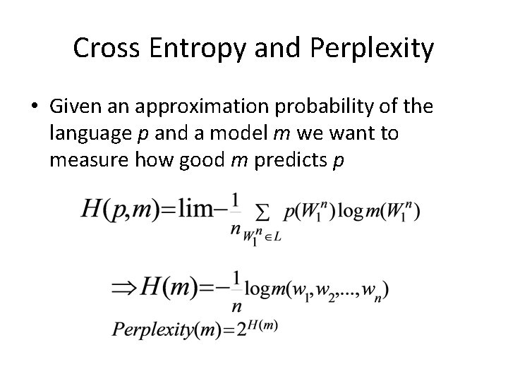
Cross Entropy and Perplexity • Given an approximation probability of the language p and a model m we want to measure how good m predicts p

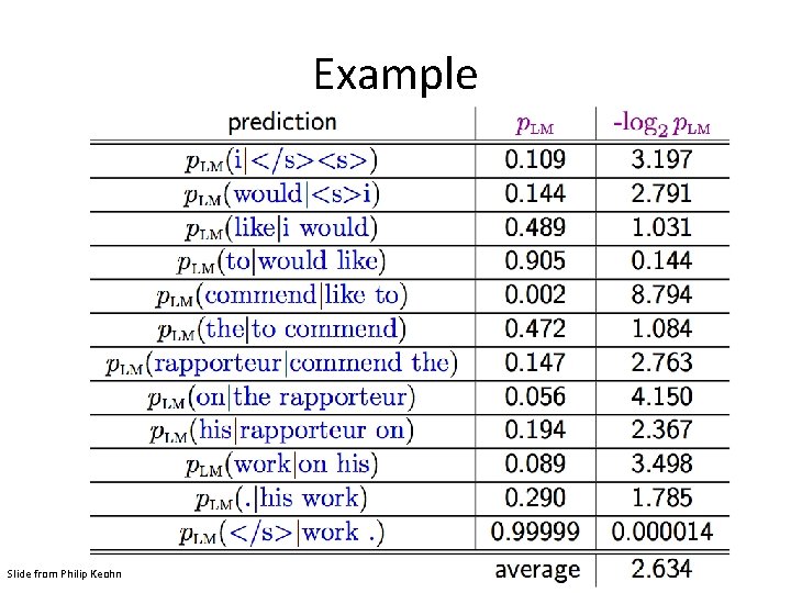
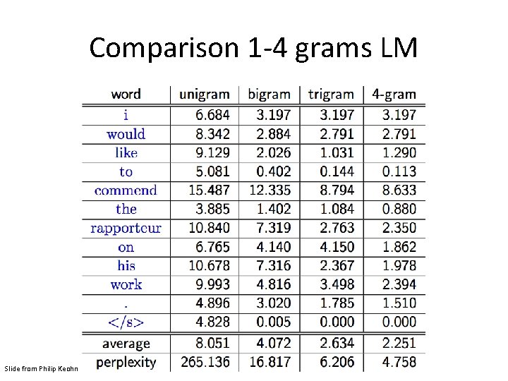
Perplexity • Better models m of the unknown distribution p will tend to assign higher probabilities m(xi) to the test events. Thus, they have lower perplexity: they are less surprised by the test sample

Example Slide from Philip Keohn

Comparison 1 -4 grams LM Slide from Philip Keohn

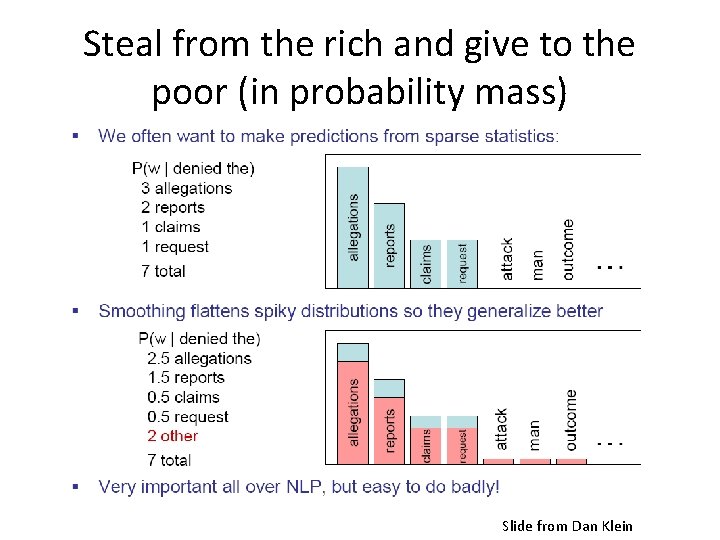
Smoothing • Words follow a Zipfian distribution – Small number of words occur very frequently – A large number are seen only once • Zero probabilities on one bigram cause a zero probability on the entire sentence • So…. how do we estimate the likelihood of unseen n-grams?

Steal from the rich and give to the poor (in probability mass) Slide from Dan Klein

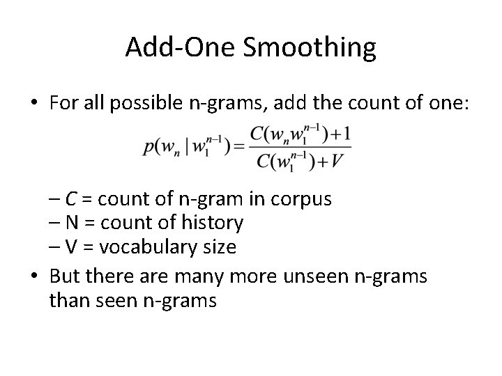
Add-One Smoothing • For all possible n-grams, add the count of one: – C = count of n-gram in corpus – N = count of history – V = vocabulary size • But there are many more unseen n-grams than seen n-grams

Add-One Smoothing 2 nd word 1 st word unsmoothed bigram counts: unsmoothed normalized bigram probabilities: Vocabulary = 1616

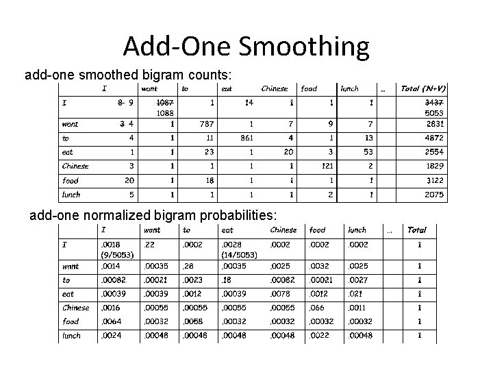
Add-One Smoothing add-one smoothed bigram counts: add-one normalized bigram probabilities:

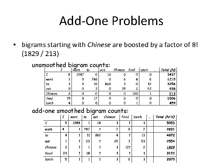
Add-One Problems • bigrams starting with Chinese are boosted by a factor of 8! (1829 / 213) unsmoothed bigram counts: add-one smoothed bigram counts:

Add-One Problems • Every previously unseen n-gram is given a low probability, but there are so many of them that too much probability mass is given to unseen events • Adding 1 to frequent bigram, does not change much, but adding 1 to low bigrams (including unseen ones) boosts them too much! • In NLP applications that are very sparse, Add-One actually gives far too much of the probability space to unseen events

Witten-Bell Smoothing • Intuition: – An unseen n-gram is one that just did not occur yet – When it does happen, it will be its first occurrence – So give to unseen n-grams the probability of seeing a new n-gram

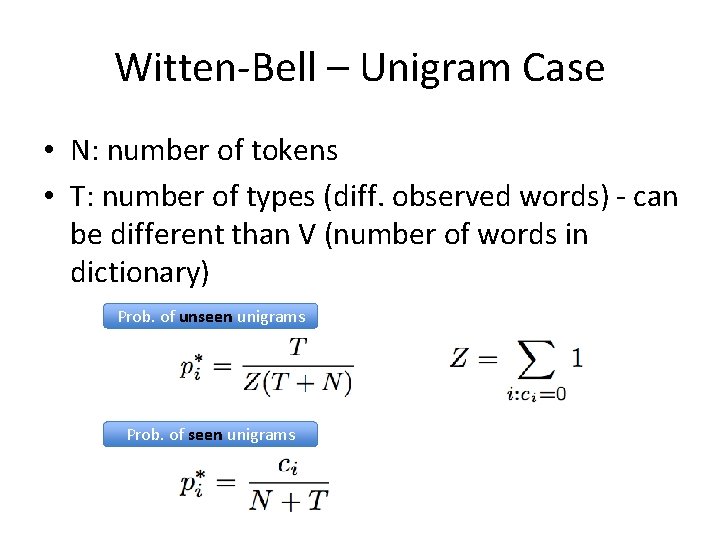
Witten-Bell – Unigram Case • N: number of tokens • T: number of types (diff. observed words) - can be different than V (number of words in dictionary) Prob. of unseen unigrams Prob. of seen unigrams

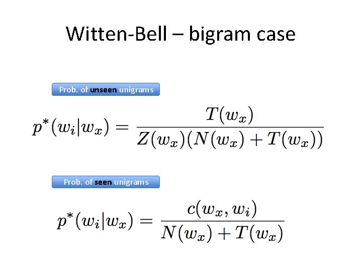
Witten-Bell – bigram case Prob. of unseen unigrams Prob. of seen unigrams

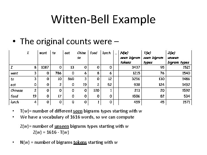
Witten-Bell Example • The original counts were – • • T(w)= number of different seen bigrams types starting with w We have a vocabulary of 1616 words, so we can compute Z(w)= number of unseen bigrams types starting with w Z(w) = 1616 - T(w) • N(w) = number of bigrams tokens starting with w

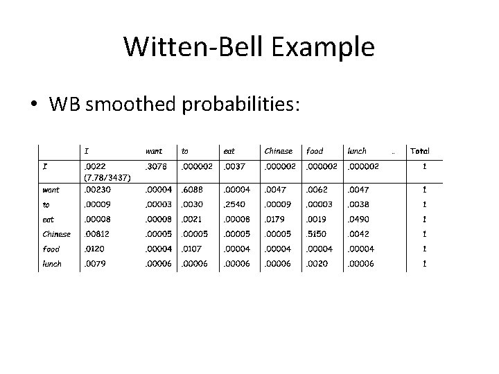
Witten-Bell Example • WB smoothed probabilities:

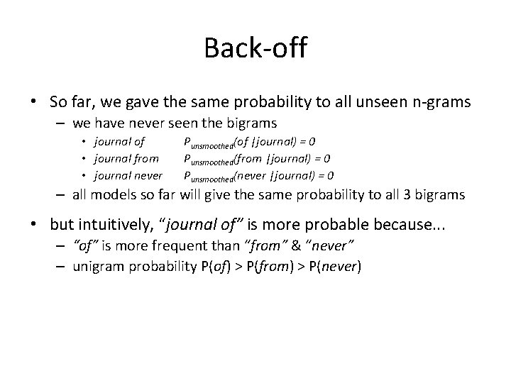
Back-off • So far, we gave the same probability to all unseen n-grams – we have never seen the bigrams • journal of • journal from • journal never Punsmoothed(of |journal) = 0 Punsmoothed(from |journal) = 0 Punsmoothed(never |journal) = 0 – all models so far will give the same probability to all 3 bigrams • but intuitively, “journal of” is more probable because. . . – “of” is more frequent than “from” & “never” – unigram probability P(of) > P(from) > P(never)

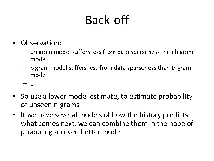
Back-off • Observation: – unigram model suffers less from data sparseness than bigram model – bigram model suffers less from data sparseness than trigram model – … • So use a lower model estimate, to estimate probability of unseen n-grams • If we have several models of how the history predicts what comes next, we can combine them in the hope of producing an even better model

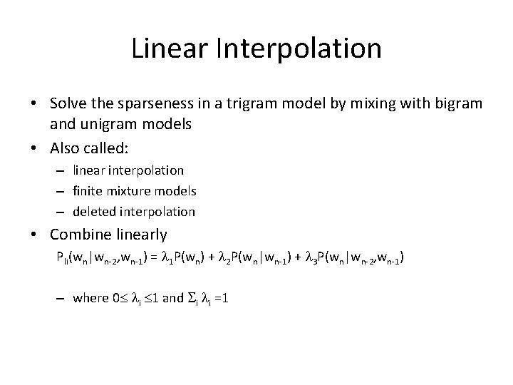
Linear Interpolation • Solve the sparseness in a trigram model by mixing with bigram and unigram models • Also called: – linear interpolation – finite mixture models – deleted interpolation • Combine linearly Pli(wn|wn-2, wn-1) = 1 P(wn) + 2 P(wn|wn-1) + 3 P(wn|wn-2, wn-1) – where 0 i 1 and i i =1

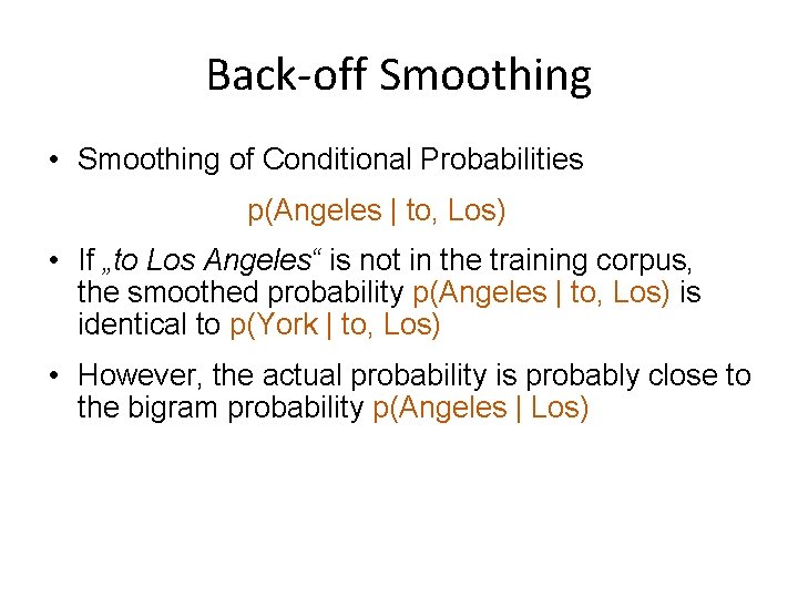
Back-off Smoothing • Smoothing of Conditional Probabilities p(Angeles | to, Los) • If „to Los Angeles“ is not in the training corpus, the smoothed probability p(Angeles | to, Los) is identical to p(York | to, Los) • However, the actual probability is probably close to the bigram probability p(Angeles | Los)

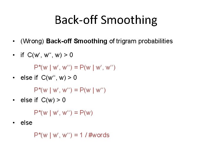
Back-off Smoothing • (Wrong) Back-off Smoothing of trigram probabilities • if C(w‘, w‘‘, w) > 0 P*(w | w‘, w‘‘) = P(w | w‘, w‘‘) • else if C(w‘‘, w) > 0 P*(w | w‘, w‘‘) = P(w | w‘‘) • else if C(w) > 0 P*(w | w‘, w‘‘) = P(w) • else P*(w | w‘, w‘‘) = 1 / #words

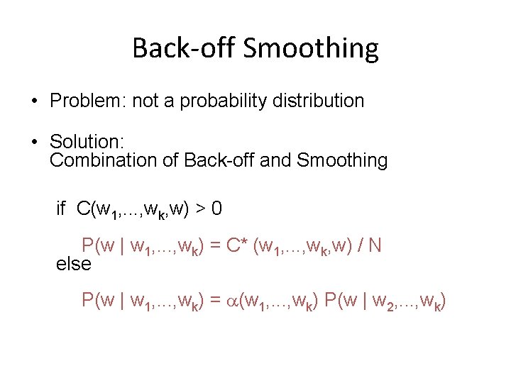
Back-off Smoothing • Problem: not a probability distribution • Solution: Combination of Back-off and Smoothing if C(w 1, . . . , wk, w) > 0 P(w | w 1, . . . , wk) = C* (w 1, . . . , wk, w) / N else P(w | w 1, . . . , wk) = (w 1, . . . , wk) P(w | w 2, . . . , wk)