National Income Equilibrium 1 BUSINESS CYCLE Aggregate Econ

National Income Equilibrium 1

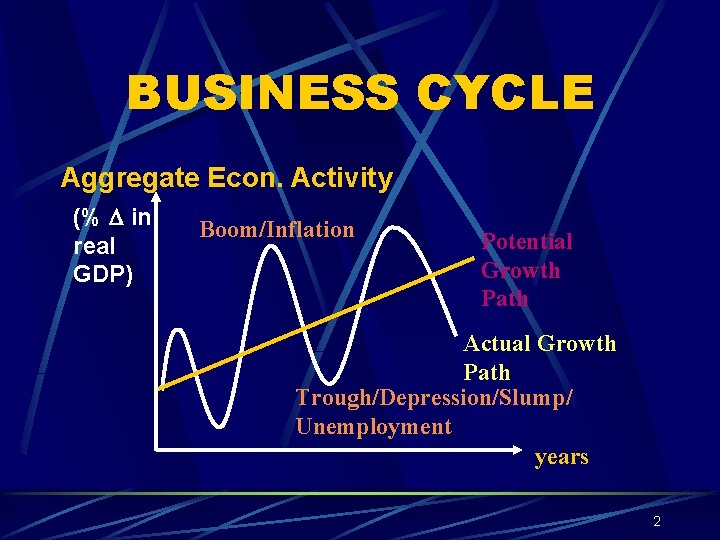
BUSINESS CYCLE Aggregate Econ. Activity (% in real GDP) Boom/Inflation Potential Growth Path Actual Growth Path Trough/Depression/Slump/ Unemployment years 2

NATIONAL INCOME EQUILIBRIUM Keynes argued that “an economy could reach equilibrium but not necessarily at the full employment. ” 3

Equilibrium and Full-employment Equilibrium will occur when there is no tendency for an economy to change. It refers to a situation when all consumers and firms have no incentive to change their behaviour. Full employment equilibrium is the situation of equilibrium in an economy at the best efficient and full utilization of resources. “An economy can be at the equilibrium but not always to be at full-employment. ” 4

Two approaches: To Determine National Income Equilibrium: 1. Total Approach or Income. Expenditure Approach 2. Injection-Leakage Approach. 5

i) Total Approach: Equilibrium may occur when planned aggregate expenditure is equivalent to planned output. (AD = AS) (aggregate demand = aggregate supply). 6

i) Leakage-Injection Approach: Equilibrium also can be determined when: INJECTION = LEAKAGE Ø Injections are additional spending from: gross investments (I), government purchases (G) and exports (X). Ø Leakages are withdrawals from: savings (S), tax payment (T) and imports (M). So, at equilibrium, (I+G+X = S+T+M) (INJECTION = LEAKAGE) 7

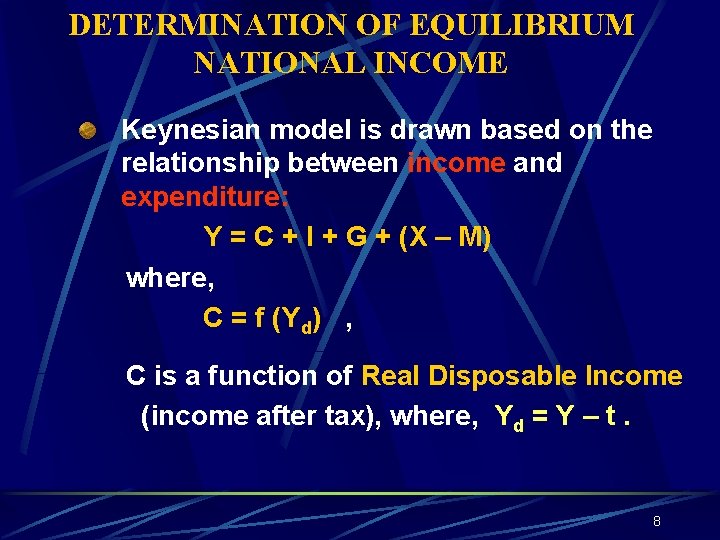
DETERMINATION OF EQUILIBRIUM NATIONAL INCOME Keynesian model is drawn based on the relationship between income and expenditure: Y = C + I + G + (X – M) where, C = f (Yd) , C is a function of Real Disposable Income (income after tax), where, Yd = Y – t. 8

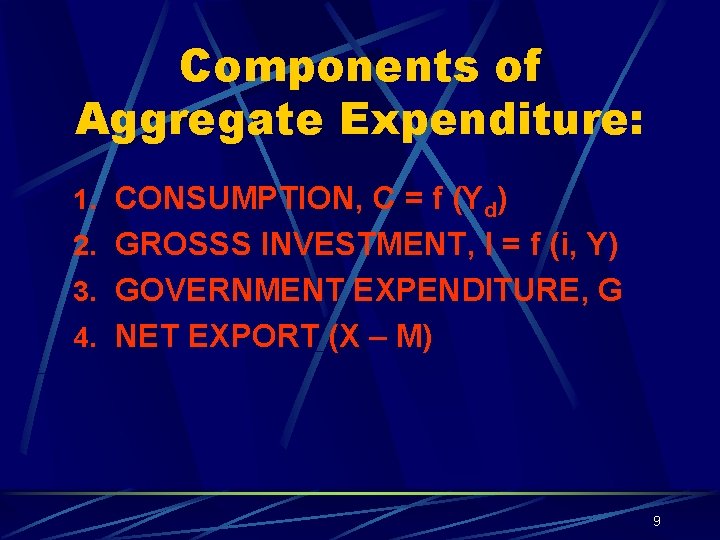
Components of Aggregate Expenditure: 1. CONSUMPTION, C = f (Yd) 2. GROSSS INVESTMENT, I = f (i, Y) 3. GOVERNMENT EXPENDITURE, G 4. NET EXPORT (X – M) 9

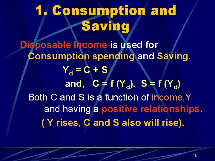
1. Consumption and Saving Disposable Income is used for Consumption spending and Saving. Yd = C + S and, C = f (Yd), S = f (Yd) Both C and S is a function of income, Y and having a positive relationships. ( Y rises, C and S also will rise). 10

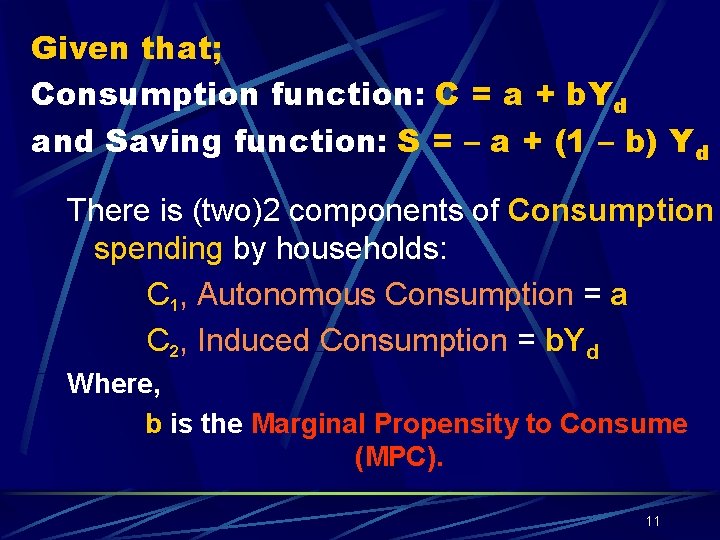
Given that; Consumption function: C = a + b. Yd and Saving function: S = – a + (1 – b) Yd There is (two)2 components of Consumption spending by households: C 1, Autonomous Consumption = a C 2, Induced Consumption = b. Yd Where, b is the Marginal Propensity to Consume (MPC). 11

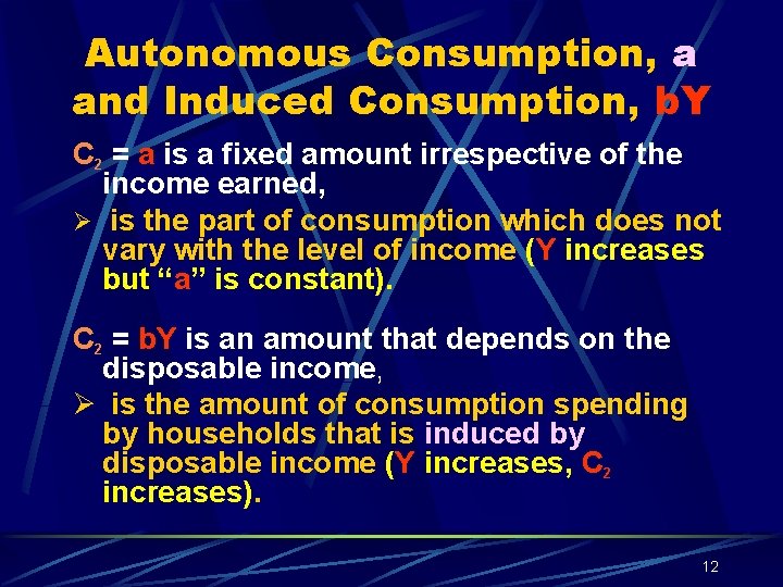
Autonomous Consumption, a and Induced Consumption, b. Y C 2 = a is a fixed amount irrespective of the income earned, Ø is the part of consumption which does not vary with the level of income (Y increases but “a” is constant). C 2 = b. Y is an amount that depends on the disposable income, Ø is the amount of consumption spending by households that is induced by disposable income (Y increases, C 2 increases). 12

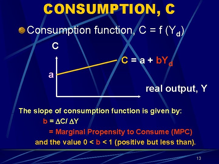
CONSUMPTION, C Consumption function, C = f (Yd) C C = a + b. Yd a real output, Y The slope of consumption function is given by: b = C/ Y = Marginal Propensity to Consume (MPC) and the value 0 < b < 1 (positive but less than). 13

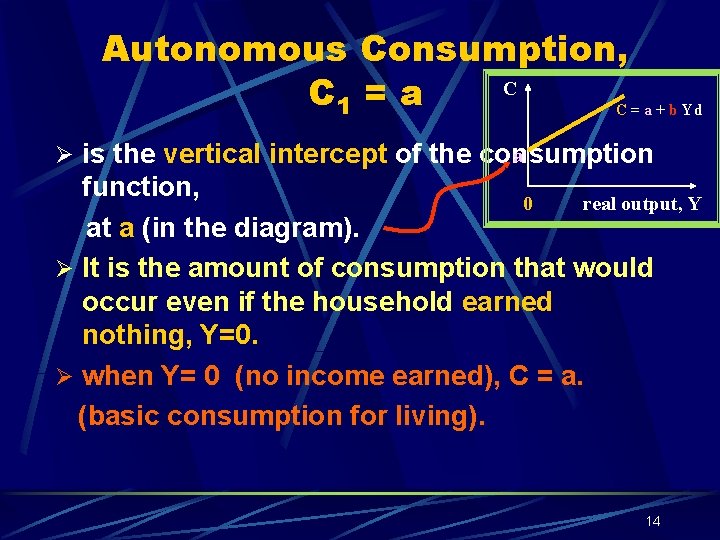
Autonomous Consumption, C C 1 = a C = a + b Yd a Ø is the vertical intercept of the consumption function, 0 real output, Y at a (in the diagram). Ø It is the amount of consumption that would occur even if the household earned nothing, Y=0. Ø when Y= 0 (no income earned), C = a. (basic consumption for living). 14

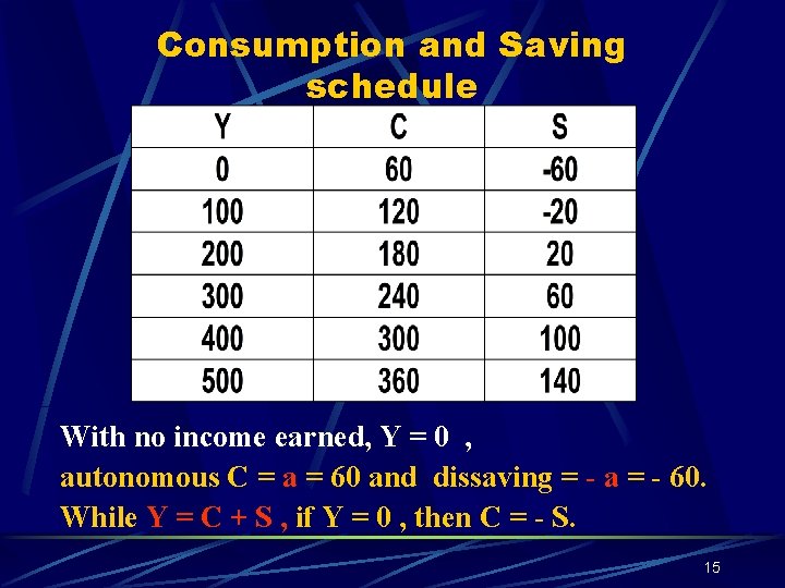
Consumption and Saving schedule With no income earned, Y = 0 , autonomous C = a = 60 and dissaving = - a = - 60. While Y = C + S , if Y = 0 , then C = - S. 15

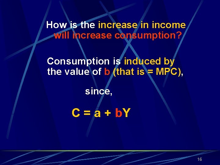
How is the increase in income will increase consumption? Consumption is induced by the value of b (that is = MPC), since, C = a + b. Y 16

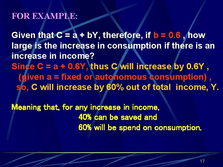
FOR EXAMPLE: Given that C = a + b. Y, therefore, if b = 0. 6 , how large is the increase in consumption if there is an increase in income? Since C = a + 0. 6 Y, thus C will increase by 0. 6 Y , (given a = fixed or autonomous consumption) , so, C will increase by 60% out of total income, Y. Meaning that, for any increase in income, 40% can be saved and 60% will be spend on consumption. 17

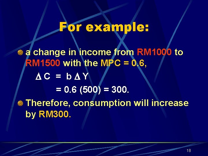
For example: a change in income from RM 1000 to RM 1500 with the MPC = 0. 6, C = b Y = 0. 6 (500) = 300. Therefore, consumption will increase by RM 300. 18

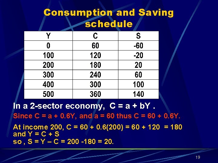
Consumption and Saving schedule In a 2 -sector economy, C = a + b. Y. Since C = a + 0. 6 Y, and a = 60 thus C = 60 + 0. 6 Y. At income 200, C = 60 + 0. 6(200) = 60 + 120 = 180 and Y = C + S so , S = Y – C = 200 -180 = 20. 19

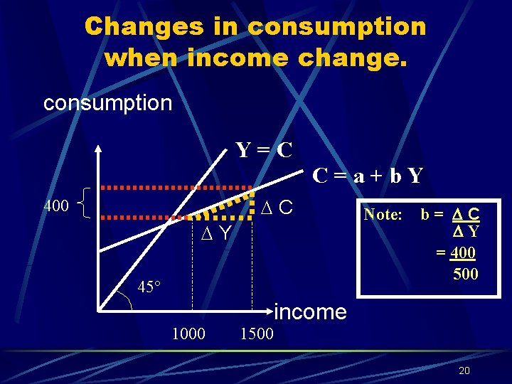
Changes in consumption when income change. consumption Y=C C=a+b. Y C 400 Y 45° 1000 1500 Note: b= C Y = 400 500 income 20

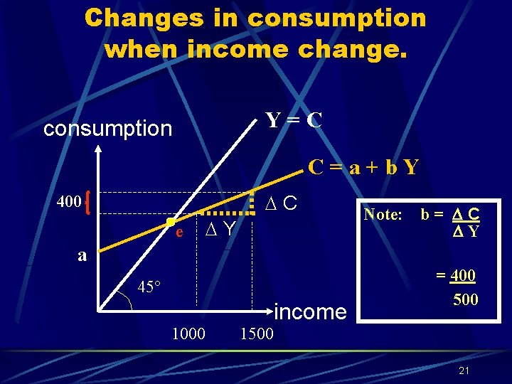
Changes in consumption when income change. Y=C consumption C=a+b. Y C 400 e Y Note: b= C Y a 45° 1000 1500 income = 400 500 21

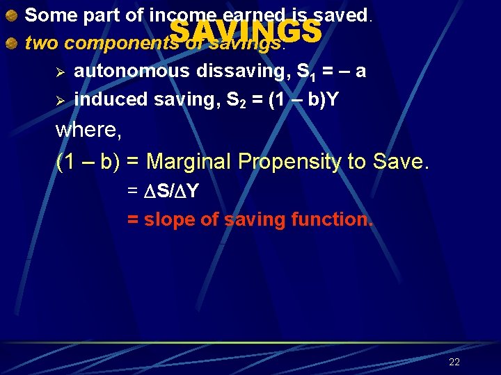
Some part of income earned is saved. SAVINGS two components of savings: Ø autonomous dissaving, S 1 = – a Ø induced saving, S 2 = (1 – b)Y where, (1 – b) = Marginal Propensity to Save. = S/ Y = slope of saving function. 22

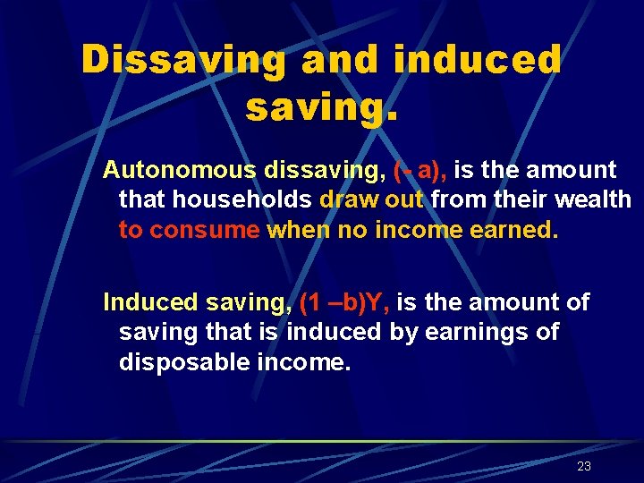
Dissaving and induced saving. Autonomous dissaving, (- a), is the amount that households draw out from their wealth to consume when no income earned. Induced saving, (1 –b)Y, is the amount of saving that is induced by earnings of disposable income. 23

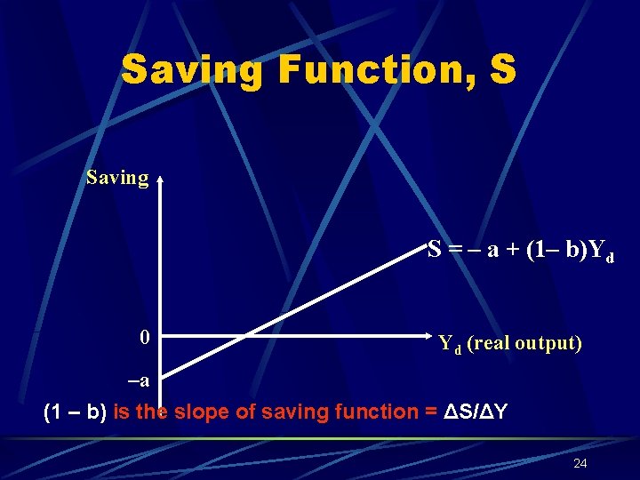
Saving Function, S Saving S = – a + (1– b)Yd 0 Yd (real output) –a (1 – b) is the slope of saving function = ΔS/ΔY 24

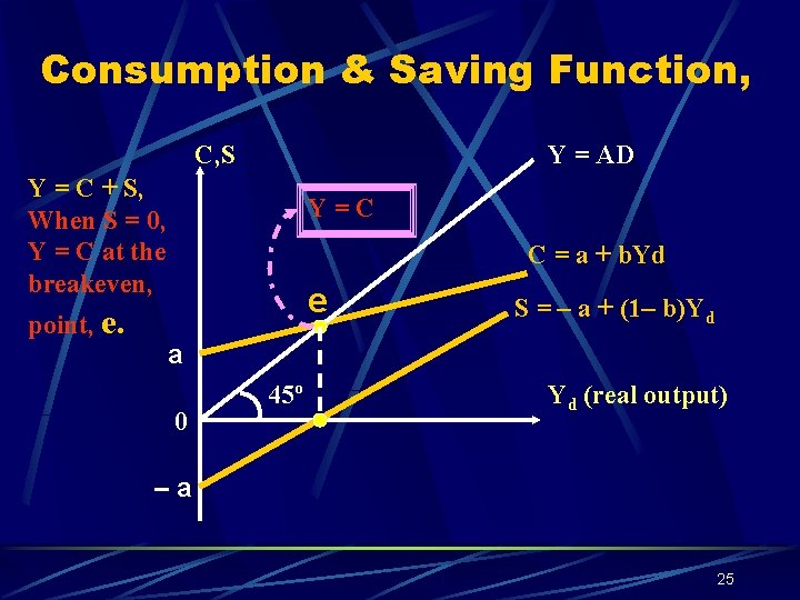
Consumption & Saving Function, C, S Y = AD Y = C + S, When S = 0, Y = C at the breakeven, point, e. Y=C C = a + b. Yd e S = – a + (1– b)Yd a 0 45º Yd (real output) –a 25

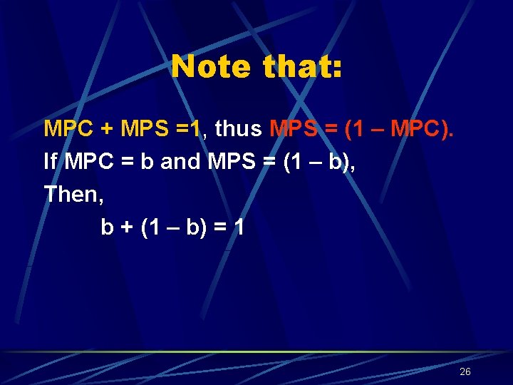
Note that: MPC + MPS =1, thus MPS = (1 – MPC). If MPC = b and MPS = (1 – b), Then, b + (1 – b) = 1 26

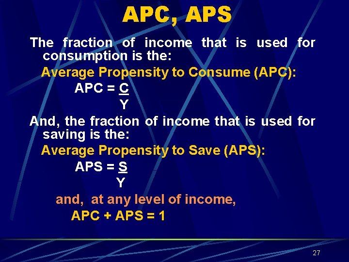
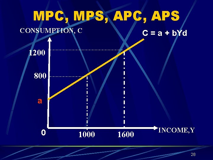
APC, APS The fraction of income that is used for consumption is the: Average Propensity to Consume (APC): APC = C Y And, the fraction of income that is used for saving is the: Average Propensity to Save (APS): APS = S Y and, at any level of income, APC + APS = 1 27

MPC, MPS, APC, APS CONSUMPTION, C C = a + b. Yd 1200 800 a 0 1000 1600 INCOME, Y 28

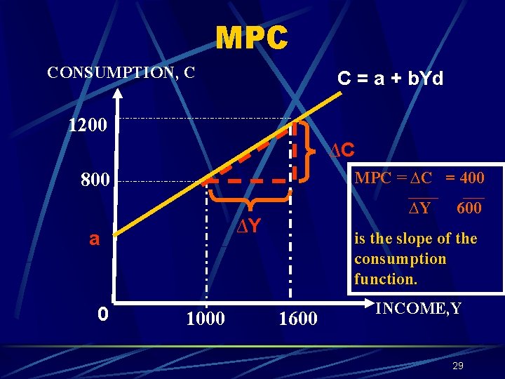
MPC CONSUMPTION, C C = a + b. Yd 1200 ∆C MPC = ∆C = 400 800 ∆Y a 0 ∆Y 1000 600 is the slope of the consumption function. 1600 INCOME, Y 29

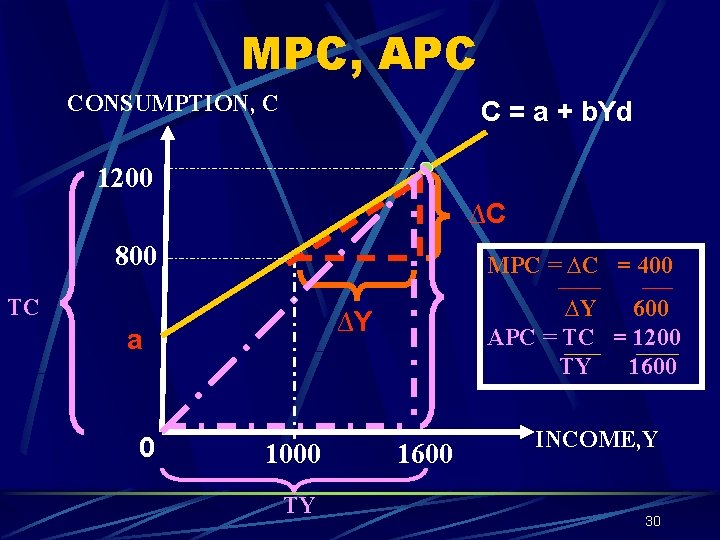
MPC, APC CONSUMPTION, C C = a + b. Yd 1200 ∆C 800 MPC = ∆C = 400 a ∆Y 600 APC = TC = 1200 TY 1600 TC 0 ∆Y 1000 TY 1600 INCOME, Y 30

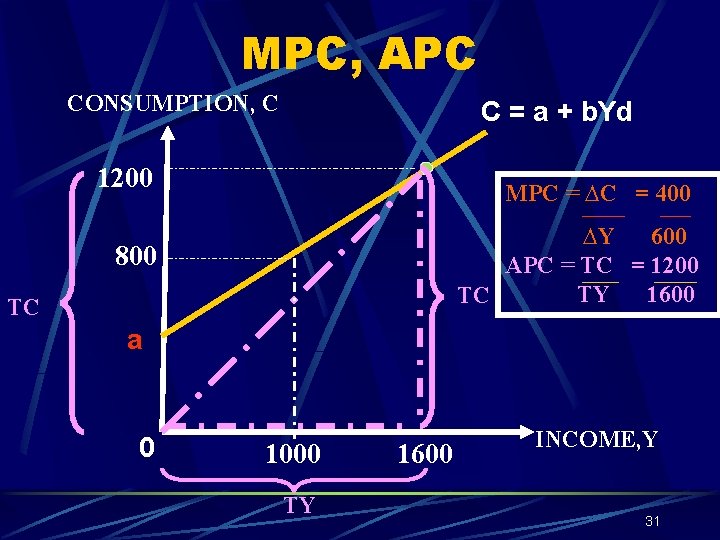
MPC, APC CONSUMPTION, C C = a + b. Yd 1200 MPC = ∆C = 400 ∆Y 600 APC = TC = 1200 TY 1600 TC 800 TC a 0 1000 TY 1600 INCOME, Y 31

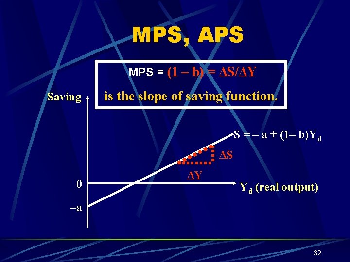
MPS, APS MPS = (1 – b) = ΔS/ΔY Saving is the slope of saving function. S = – a + (1– b)Yd ΔS 0 ΔY Yd (real output) –a 32

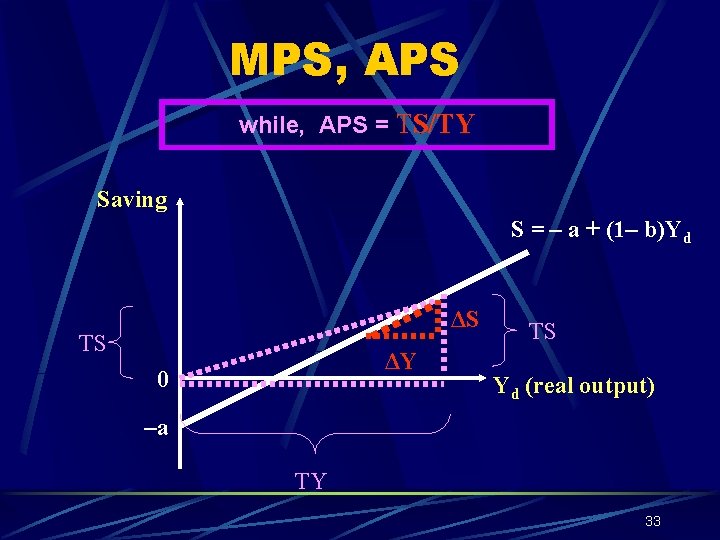
MPS, APS while, APS = TS/TY Saving S = – a + (1– b)Yd ΔS TS ΔY 0 TS Yd (real output) –a TY 33

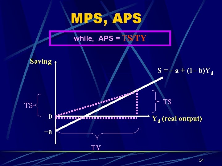
MPS, APS while, APS = TS/TY Saving S = – a + (1– b)Yd TS TS 0 Yd (real output) –a TY 34

APC, APS changes with income; MPC, MPS are constant. APC falls and APS will rise as income increases. - because as income increases, households consumption will rise but with a smaller percentage compared to the increase in income, while saving will rise with a larger percentage instead. While MPC and MPS is assume constant as long as the slopes of the consumption and saving curves are constant or assume to be straight lines. 35

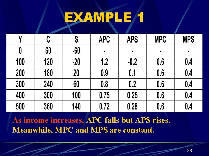
EXAMPLE 1 As income increases, APC falls but APS rises. Meanwhile, MPC and MPS are constant. 36

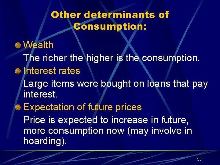
Other determinants of Consumption: Wealth The richer the higher is the consumption. Interest rates Large items were bought on loans that pay interest. Expectation of future prices Price is expected to increase in future, more consumption now (may involve in hoarding). 37

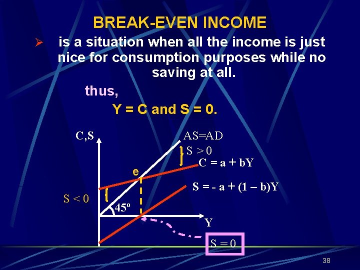
BREAK-EVEN INCOME Ø is a situation when all the income is just nice for consumption purposes while no saving at all. thus, Y = C and S = 0. C, S e S<0 AS=AD S>0 C = a + b. Y S = - a + (1 – b)Y 45º Y S=0 38

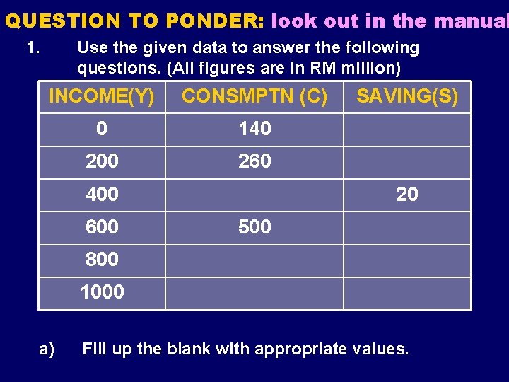
QUESTION TO PONDER: look out in the manual 1. Use the given data to answer the following questions. (All figures are in RM million) INCOME(Y) CONSMPTN (C) 0 140 200 260 400 600 SAVING(S) 20 500 800 1000 a) Fill up the blank with appropriate values.

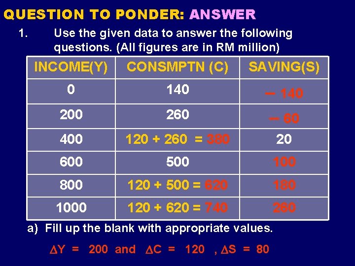
QUESTION TO PONDER: ANSWER 1. Use the given data to answer the following questions. (All figures are in RM million) INCOME(Y) CONSMPTN (C) SAVING(S) 0 140 200 260 140 60 400 120 + 260 = 380 20 600 500 100 800 120 + 500 = 620 180 1000 120 + 620 = 740 260 a) Fill up the blank with appropriate values. Y = 200 and C = 120 , S = 80

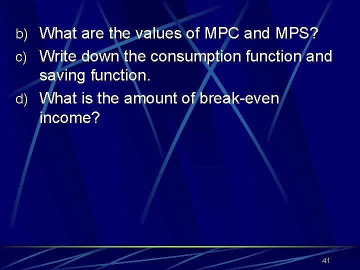
b) What are the values of MPC and MPS? c) Write down the consumption function and saving function. d) What is the amount of break-even income? 41

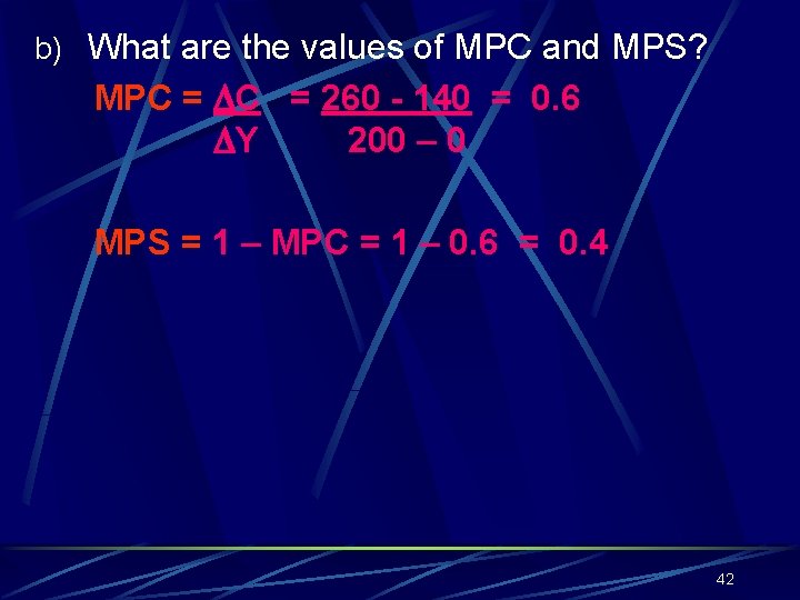
b) What are the values of MPC and MPS? MPC = 260 - 140 = 0. 6 Y 200 – 0 MPS = 1 – MPC = 1 – 0. 6 = 0. 4 42

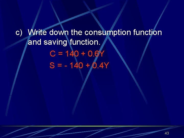
c) Write down the consumption function and saving function. C = 140 + 0. 6 Y S = - 140 + 0. 4 Y 43

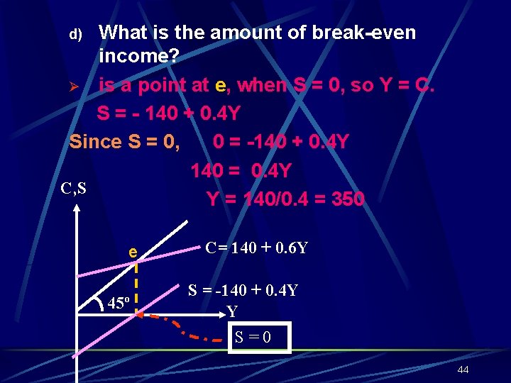
What is the amount of break-even income? Ø is a point at e, when S = 0, so Y = C. S = - 140 + 0. 4 Y Since S = 0, 0 = -140 + 0. 4 Y 140 = 0. 4 Y C, S Y = 140/0. 4 = 350 d) e 45º C= 140 + 0. 6 Y S = -140 + 0. 4 Y Y S=0 44

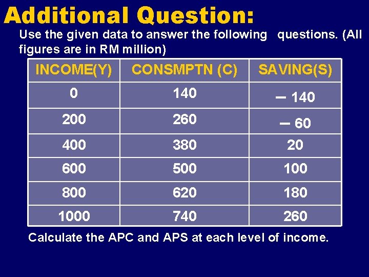
Additional Question: Use the given data to answer the following questions. (All figures are in RM million) INCOME(Y) CONSMPTN (C) SAVING(S) 0 140 200 260 140 60 400 380 20 600 500 100 800 620 180 1000 740 260 Calculate the APC and APS at each level of income.

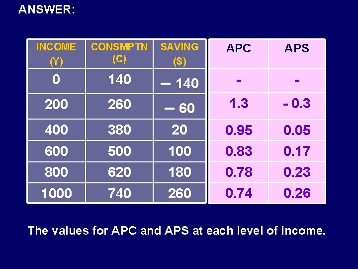
ANSWER: INCOME (Y) CONSMPTN (C) SAVING (S) APC APS 0 140 - - 200 260 140 60 1. 3 - 0. 3 400 380 20 0. 95 0. 05 600 500 100 800 620 180 1000 740 260 0. 83 0. 78 0. 74 0. 17 0. 23 0. 26 The values for APC and APS at each level of income.

2. INVESTMENT Definition: Investment is defined as the spending or purchase of plants, machineries, buildings and inventories by firms for the purpose of producing goods and services. 47

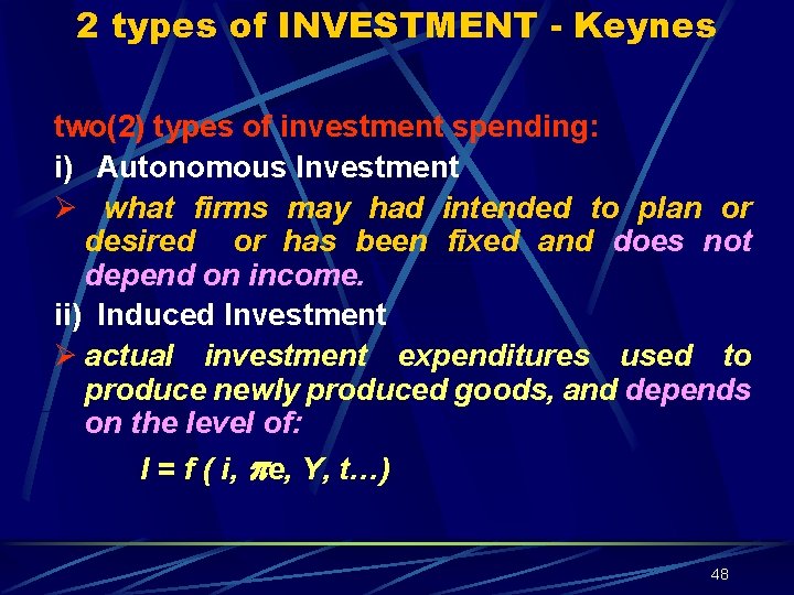
2 types of INVESTMENT - Keynes two(2) types of investment spending: i) Autonomous Investment Ø what firms may had intended to plan or desired or has been fixed and does not depend on income. ii) Induced Investment Ø actual investment expenditures used to produce newly produced goods, and depends on the level of: I = f ( i, e, Y, t…) 48

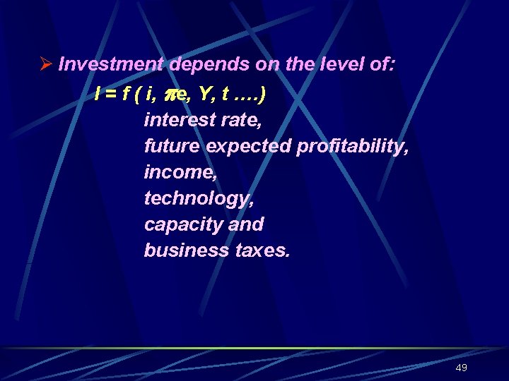
Ø Investment depends on the level of: I = f ( i, e, Y, t …. ) interest rate, future expected profitability, income, technology, capacity and business taxes. 49

1. Autonomous Investment As assume by Keynes; - is a fixed investment that does not change with the change in income, but ; there will be a shift in the autonomous horizontal function, up or down when there’re other factors that affect it. 50

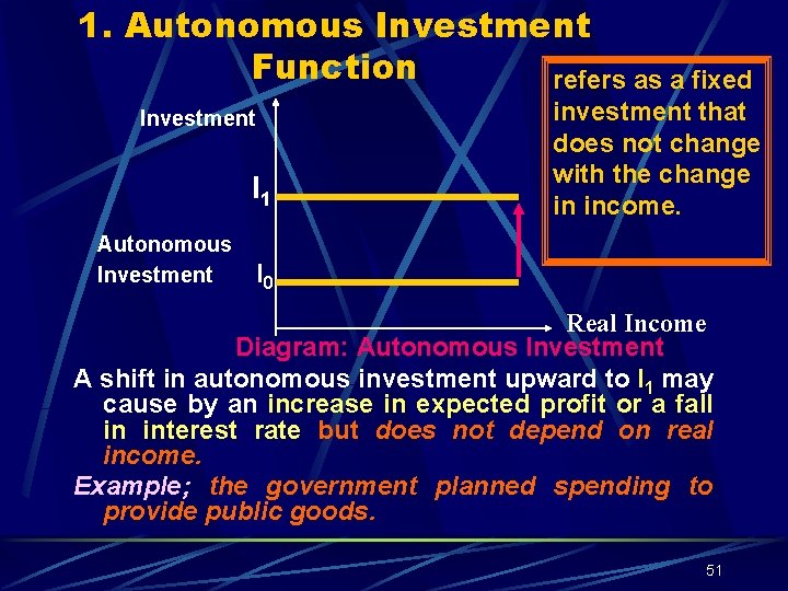
1. Autonomous Investment Function refers as a fixed Investment I 1 Autonomous Investment investment that does not change with the change in income. I 0 Real Income Diagram: Autonomous Investment A shift in autonomous investment upward to I 1 may cause by an increase in expected profit or a fall in interest rate but does not depend on real income. Example; the government planned spending to provide public goods. 51

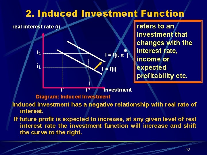
2. Induced Investment Function real interest rate (i) i 2 i 1 e I = f(i, ) I = f(i) refers to an investment that changes with the interest rate, income or expected profitability etc. I’ I’’ Investment Diagram: Induced Investment Induced investment has a negative relationship with real rate of interest. If future profit is expected to increase, at any given level of real interest rate the investment function will increase and shift the curve to the right. 52

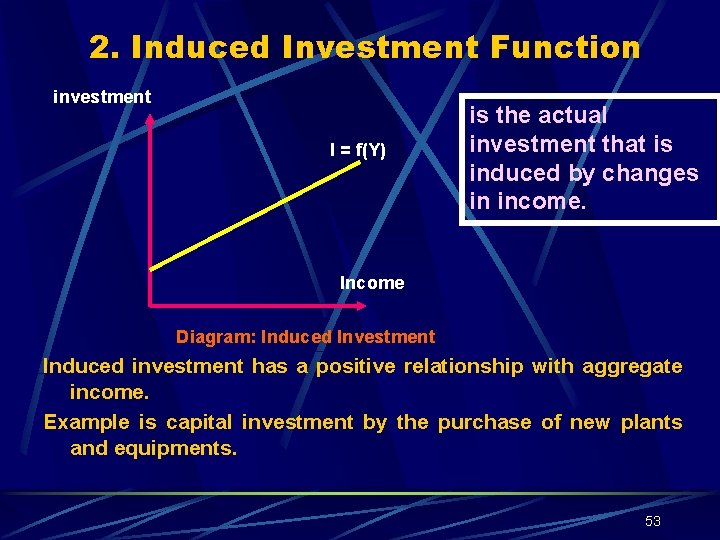
2. Induced Investment Function investment I = f(Y) is the actual investment that is induced by changes in income. Income Diagram: Induced Investment Induced investment has a positive relationship with aggregate income. Example is capital investment by the purchase of new plants and equipments. 53

Factors that influence Investment are: Income II. Expected returns III. Viability of the projects. IV. Facilities available or provided by the government. V. The respond of market demand. VI. Availability of fund. I. 54

Investment and Saving Investment is an injection: could increase aggregate expenditure (AD) and boost up economic growth (income). Investment spending will multiply through the multiplier effect to increase income. Saving is a leakage: could lower aggregate expenditure (AD) and income. Saving becomes an outflow of money (leakage) from an economy. It becomes a stock of money that is not spent. At equilibrium, Saving will be equal to Investment, (S=I) 55

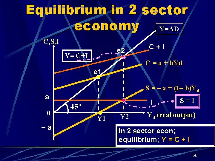
Equilibrium in 2 sector economy Y=AD C, S, I e 2 Y= C+I C = a + b. Yd e 1 S = – a + (1– b)Yd a 0 –a I 45º Y 1 Y 2 S=I Yd (real output) In 2 sector econ; equilibrium; Y = C + I 56

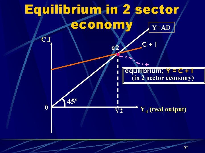
Equilibrium in 2 sector economy Y=AD C, I e 2 C+I equilibrium; Y = C + I (in 2 sector economy) 0 45º Y 2 Yd (real output) 57

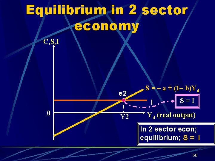
Equilibrium in 2 sector economy C, S, I e 2 S = – a + (1– b)Yd I 0 Y 2 S=I Yd (real output) In 2 sector econ; equilibrium; S = I 58

QUESTION TO PONDER 1 e) If investment is RM 150 millions, calculate the equilibrium income and sketch a diagram to show this. I = 150 C = 140 + 0. 6 Y 59

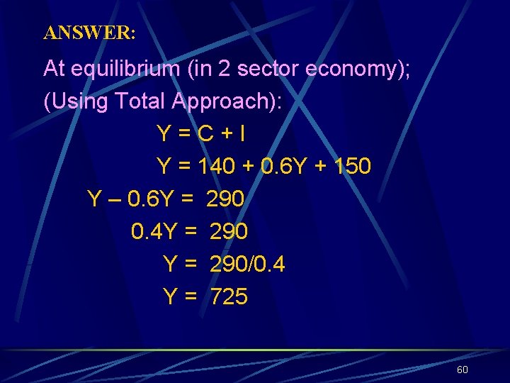
ANSWER: At equilibrium (in 2 sector economy); (Using Total Approach): Y=C+I Y = 140 + 0. 6 Y + 150 Y – 0. 6 Y = 290 0. 4 Y = 290/0. 4 Y = 725 60

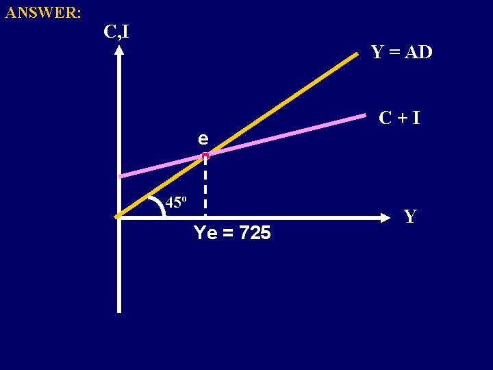
ANSWER: C, I Y = AD e 45º Ye = 725 C+I Y

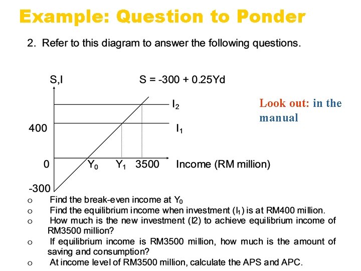
Example: Question to Ponder Look out: in the manual

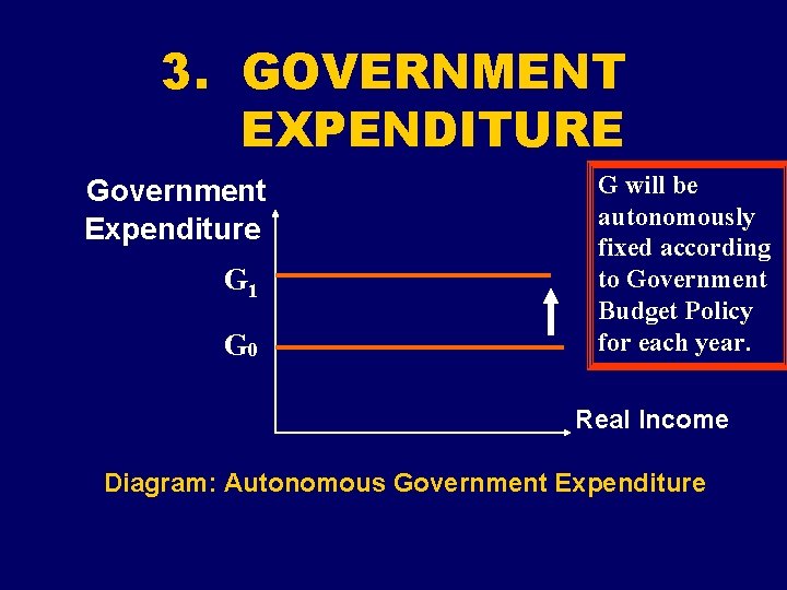
3. GOVERNMENT EXPENDITURE Government Expenditure G 1 G 0 G will be autonomously fixed according to Government Budget Policy for each year. Real Income Diagram: Autonomous Government Expenditure

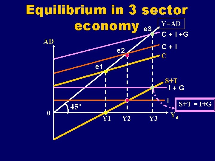
Equilibrium in 3 sector Y=AD economy e 3 C + I +G AD C+I C e 2 e 1 S+T I+G 0 I 45º Y 1 Y 2 Y 3 S+T = I+G Yd

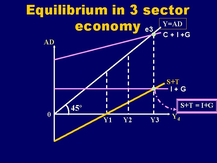
Equilibrium in 3 sector Y=AD economy e 3 C + I +G AD S+T I+G 0 S+T = I+G 45º Y 1 Y 2 Y 3 Yd

4. NET EXPORT (X – M) Export is an injection and could increase the national income through the foreign trade multiplier, but import is a leakage. Thus, net export (X-M), means the real foreign sector minus the total import of goods and services into the economy. 66

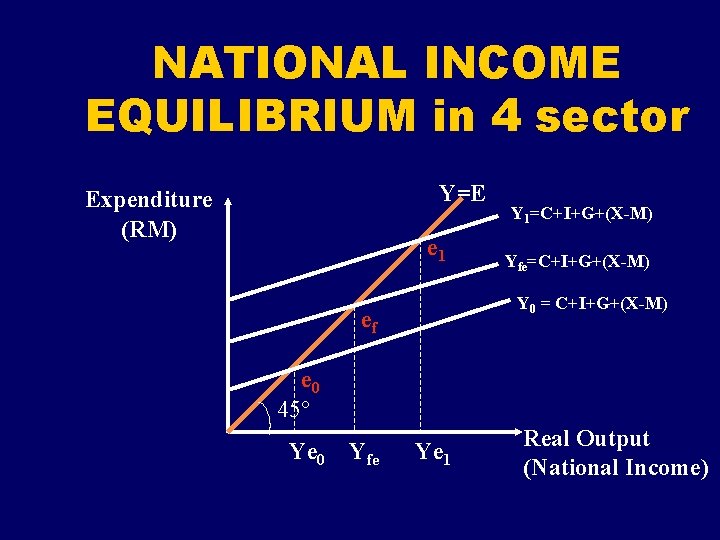
NATIONAL INCOME EQUILIBRIUM in 4 sector Y=E Expenditure (RM) e 1 Y 1=C+I+G+(X-M) Yfe=C+I+G+(X-M) Y 0 = C+I+G+(X-M) ef e 0 45° Ye 0 Yfe Ye 1 Real Output (National Income)

KEYNESIAN EQUILIBRIUM NATIONAL INCOME Ø Keynesian assume that equilibrium output can be reached not necessarily at the full-employment. - the equilibrium can be less or more than the full-employment equilibrium, causing the economy with the inflationary or deflationary-gap. 68

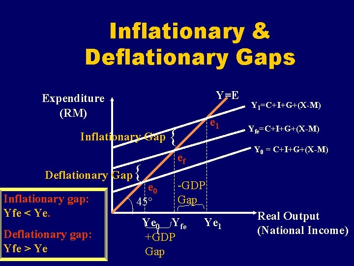
Inflationary & Deflationary Gaps Y=E Expenditure (RM) Inflationary Gap Deflationary Gap Inflationary gap: Yfe < Ye. Deflationary gap: Yfe > Ye e 0 45° e 1 Y 1=C+I+G+(X-M) Yfe=C+I+G+(X-M) Y 0 = C+I+G+(X-M) ef -GDP Gap Ye 0 Yfe +GDP Gap Ye 1 Real Output (National Income)

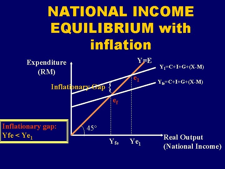
NATIONAL INCOME EQUILIBRIUM with inflation Y=E Expenditure (RM) Inflationary Gap e 1 Y 1=C+I+G+(X-M) Yfe=C+I+G+(X-M) ef Inflationary gap: Yfe < Ye 1 45° Yfe Ye 1 Real Output (National Income)

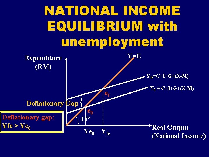
NATIONAL INCOME EQUILIBRIUM with unemployment Y=E Expenditure (RM) Yfe=C+I+G+(X-M) Deflationary Gap Deflationary gap: Yfe > Ye 0 ef Y 0 = C+I+G+(X-M) e 0 45° Ye 0 Yfe Real Output (National Income)

NATIONAL INCOME EQUILIBRIUM Y=E Expenditure (RM) e 1 Spending multiplier , ef Yfe– Y 0 Thus , Y = m G G e 0 Yfe=C+I+G 1+(X-M) Y 0 = C+I+G 0+(X-M) m = Y G = G 1 – G 0 Y 1=C+I+G 2+(X-M) 45° Y Y 0 Yfe +GDP Gap Y 1 Real Output (National Income)

MULTIPLIERS Any Injection will multiply positively, while any Leakage will multiply negatively. 73

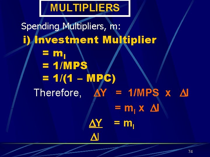
MULTIPLIERS Spending Multipliers, m: i) Investment Multiplier = m. I = 1/MPS = 1/(1 – MPC) Therefore, Y = 1/MPS x I = m I x I Y = m. I I 74

Example: Investment Multiplier Given, I = RM 10 million and MPC = 0. 75 Therefore, in the manual Y = 1/MPS x I = 1/0. 25 X 10 mil. = 40 mil. Thus, New Y = Y + 40 mil. If the initial income, Y= 2000, then New Y = 2000 + 40 = 2040 mil. 75

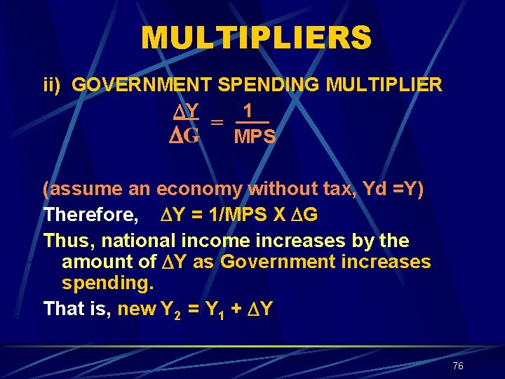
MULTIPLIERS ii) GOVERNMENT SPENDING MULTIPLIER Y 1 = G MPS (assume an economy without tax, Yd =Y) Therefore, Y = 1/MPS X G Thus, national income increases by the amount of Y as Government increases spending. That is, new Y 2 = Y 1 + Y 76

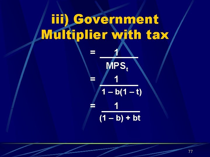
iii) Government Multiplier with tax = = 1 MPS t 1 1 – b(1 – t) = 1 (1 – b) + bt 77

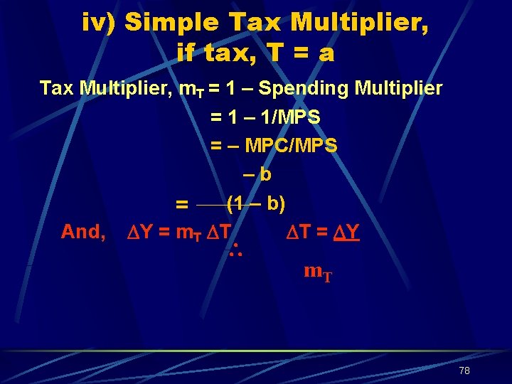
iv) Simple Tax Multiplier, if tax, T = a Tax Multiplier, m. T = 1 – Spending Multiplier = 1 – 1/MPS = – MPC/MPS –b (1 – b) = And, Y = m. T T T = Y m. T 78

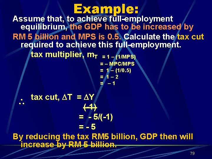
Example: Assume that, to achieve full-employment equilibrium, the GDP has to be increased by RM 5 billion and MPS is 0. 5. Calculate the tax cut required to achieve this full-employment. tax multiplier, m. T = 1 – (1/MPS) = – MPC/MPS = 1 – (1/0. 5) = 1– 2 = – 1 tax cut, T = Y (-1) = - 5/(-1) =-5 By reducing the tax RM 5 billion, GDP then will increase by RM 5 billion. 79

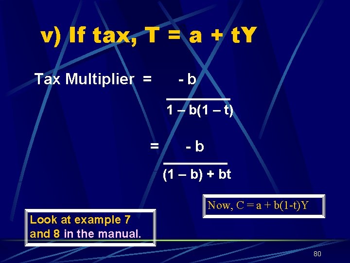
v) If tax, T = a + t. Y Tax Multiplier = -b 1 – b(1 – t) = -b (1 – b) + bt Now, C = a + b(1 -t)Y Look at example 7 and 8 in the manual. 80

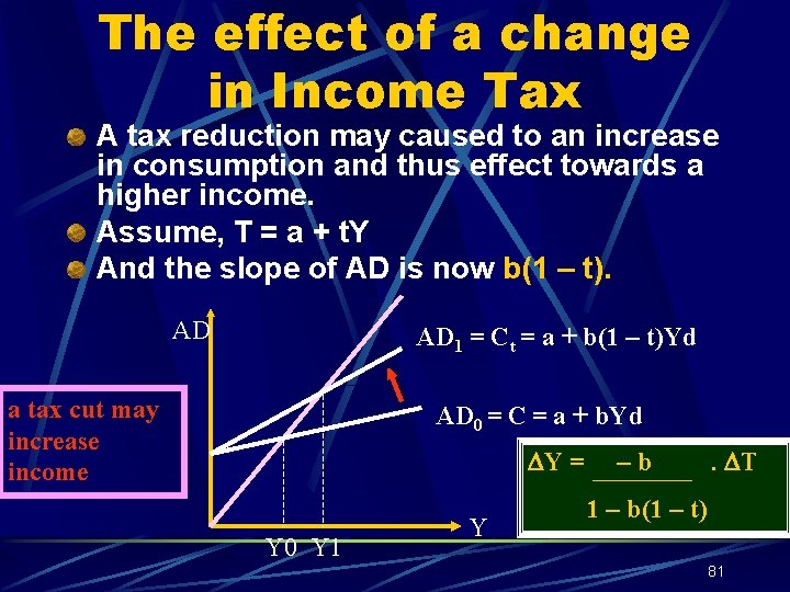
The effect of a change in Income Tax A tax reduction may caused to an increase in consumption and thus effect towards a higher income. Assume, T = a + t. Y And the slope of AD is now b(1 – t). AD AD 1 = Ct = a + b(1 – t)Yd a tax cut may increase income AD 0 = C = a + b. Yd Y = Y 0 Y 1 Y –b . T 1 – b(1 – t) 81

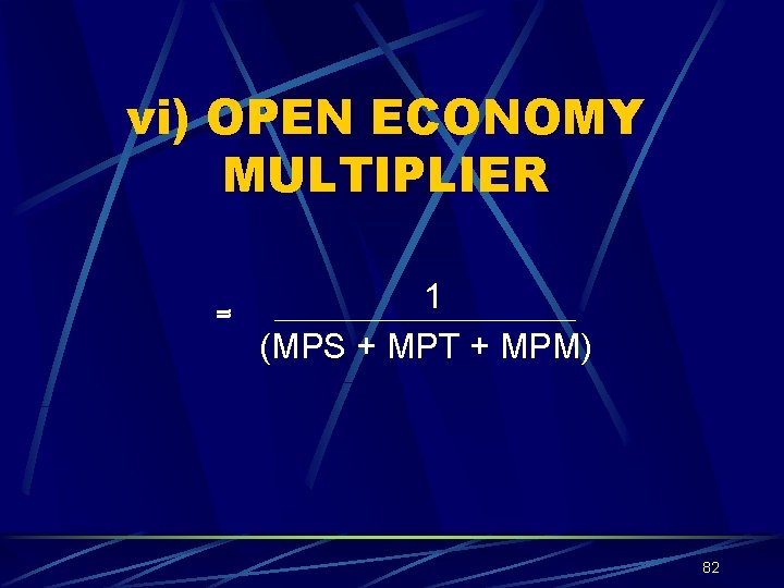
vi) OPEN ECONOMY MULTIPLIER = 1 (MPS + MPT + MPM) 82

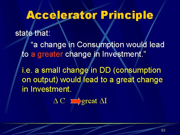
Accelerator Principle state that: “a change in Consumption would lead to a greater change in Investment. ” i. e. a small change in DD (consumption on output) would lead to a great change in Investment. ∆C great ∆I 83

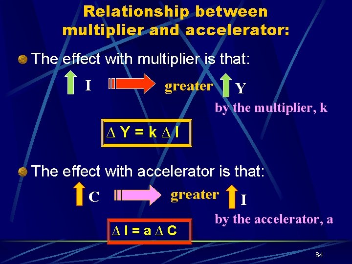
Relationship between multiplier and accelerator: The effect with multiplier is that: I greater Y by the multiplier, k ∆Y=k∆I The effect with accelerator is that: greater I C ∆I=a∆C by the accelerator, a 84

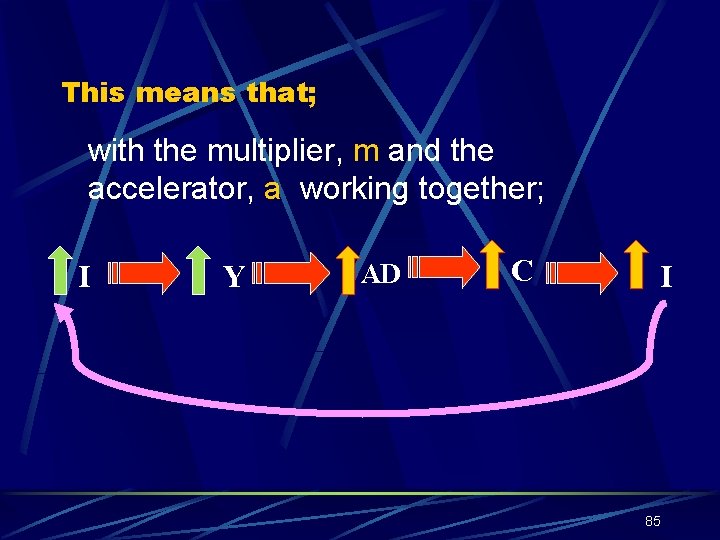
This means that; with the multiplier, m and the accelerator, a working together; I Y AD C I 85

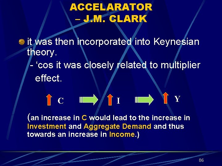
ACCELARATOR – J. M. CLARK it was then incorporated into Keynesian theory. - ‘cos it was closely related to multiplier effect. C I Y (an increase in C would lead to the increase in Investment and Aggregate Demand thus towards an increase in Income. ) 86

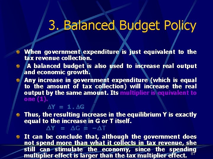
3. Balanced Budget Policy When government expenditure is just equivalent to the tax revenue collection. A balanced budget is also used to increase real output and economic growth. Any increase in government expenditure (which is equal to the amount of tax collection) will increase the real output by the same amount. Its multiplier is equivalent to one (1). Y = 1. G Thus, the resulting increase in the equilibrium Y is exactly equal to the increase in G or T itself. ∆Y = ∆G = −∆T It can be conclude that, although the government does not spend more than what it collects in tax revenue, she still can stimulate the economy, since the spending multiplier effect is larger than the tax multiplier effect. 87