n Inverse Transform Method n Composition Method n

一般隨機變數的產生方式 均勻分配以外的隨機變數通常藉由下列方 法，透過均勻亂數產生。 n Inverse Transform Method n Composition Method n Rejection (and Acceptance) Method n Alias Method n Table Method

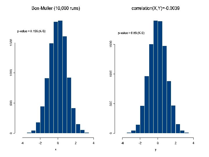
n Box and Muller(1958) The best known “exact” method for the normal distribution. n Algorithm 1. Generate U 1, U 2 ~ U(0, 1) 2. Let = 2 U 1 E = –log. U 2 & R = 3. Then X = R cos and Y = R sin are independent standard normal variables.

n Note: Using Box-Muller method with congruential generators must be careful. It is found by several researchers that a (乘數) = 131 c (增量) = 0 m (除數) = 235 would have X (– 3. 3, 3. 6). See Neave (1973) and Ripley (1987, p. 55) for further information.

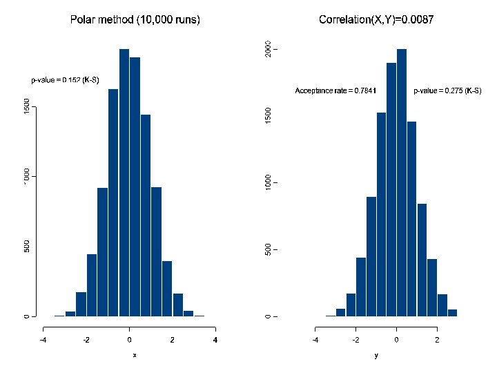
n Polar Method (recommended!) Rejection method for generating two independent normal variables. n Algorithm 1. Generate V 1, V 2 ~ U(-1, 1) retain if 2. Let 3. Then X = CV 1 and Y = CV 2 are independent standard normal variables.

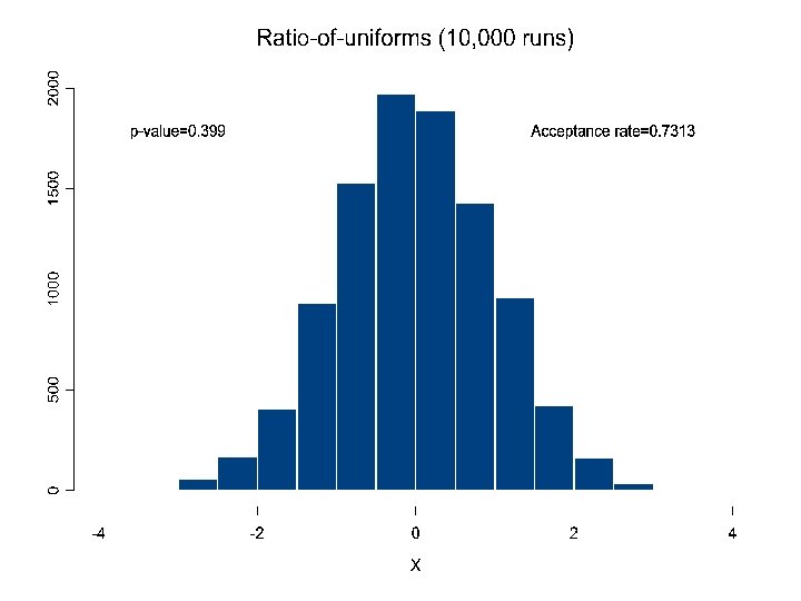
n Ratio-of-uniforms (recommended!) Similar to Polar method, Ratio-of-uniforms is a rejection method. n Algorithm 1. Generate U 1 , U 2 ~ U(0, 1), and let 2. Let X = V / U 1 , Z = X 2/4 3. Retain if Z < 1 – U 1 Suggest deleting this step! 4. Retain if 5. Then X is normally distributed.

n Ratio of Uniform (Cauchy Distribution) Ratio-of-uniforms can also be used to create random variables from Cauchy Distribution. n Algorithm 1. Generate U 1, U 2 ~ U(0, 1), and V= 2 U 2 – 1 retain if 2. Then X = V / U 1 ~ Cauchy(0, 1), i. e. g. 10, 000 runs p-value=0. 9559 (Acceptance rate = 0. 7819)

Inverse Transformation Method Generates a random number from a probability density function by solving the probability density function's variable in terms of randomly generated numbers. This is achieved as follows: We solve the inverse of the integral of our probability density function at an arbitrary point a F(a), in terms of a random number r. n We generate a unique random variable a, as follows: a = F-1(r). The foundation of this method is F(X) ~ U(0, 1) for all X. n

n Note: Usually, we only use Inversion to create simpler r. v. ’s, such as exponential distribution (i. e. Exp( ) = – log(U(0, 1)). Although Inversion is a universal method, it may be too slow (unless subprograms to calculate F-1 are available). In other words, although theoretically it is possible to create any r. v. ’s, usually there are simpler methods.

n Example 1. F(x) = x 2, 0 < x < 1 X = U 1/2. 2. Let and we want to generate the minimum and maximum of X’s. Since which means we can generate these two r. v. ’s by

n Example 3. Generate X ~ Poisson( ), i. e. where i {0, 1, 2, …}. n Algorithm: 1. Generate U 1 ~ U(0, 1) and let i = 0. 2. If let i = i + 1; Otherwise X = i. Note: This method can be used to generate any discrete distributions.

Notes: (1) If total number of classes 30, we start from the middle (or mode). (2) The expected number of trials is E(X)+1. (3) We can use “Indexed Search” to increase the efficiency: Fix m, let Step 1. Generate U~U(0, 1), let k=[m. U] & i=qk Step 2. If let i = i + 1; Otherwise X = i.

n Example 4. X ~ Poisson(10) (1) Usual method: 11 comparisons on average (2) Mode: Reduced to about 3. 54 comparisons (3) Indexed search: we choose m = 5, i. e. Under 10, 000 simulation runs (S-Plus), I found that one check on the table plus 2. 346 comparisons 3. 346 (Comparing to 3. 3 in Ripley’s book)

Composition Method n We can generate complex distribution from simpler distributions, i. e. where Fi(x) are d. f. of other variables. Or, from a conditional distribution,

n Example 1. To simulate x, where We define X 1=0. 1 for x {1, 2, …, 10} & X 2=0. 2 for x {2, 4, …, 10}. Let X= 0. 5(X 1+ X 2). n Example 2. X ~ B(5, 0. 2) Sampling on each digit:

n Example 3. Generate an r. v. X from n Algorithm: 1. Generate U 1, U 2 from U(0, 1) 2. Let Y (U 1)-1/n 3. Return X -log(U 2)/y Note:

Rejection Method Generates random numbers for a distribution function f(x). This is achieved as follows: Define a comparison function h(x) such that it encloses the desired function f(x). n Choose uniformly distributed random points under h(x). n If a point lies outside the area under f(x) reject it and choose another point. n

Illustration of the Rejection Method The following is an illustration of the rejection method using a square function for the comparison function.

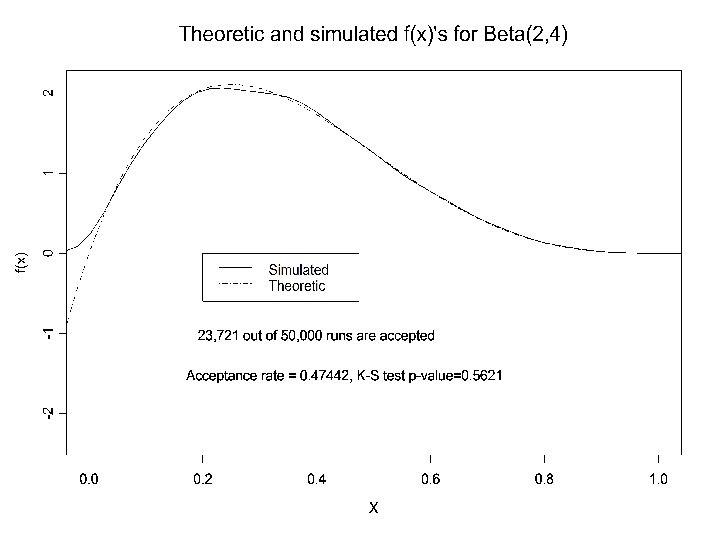
n Example 1. X ~ Beta(2, 4), i. e. E(X)=1/3, Then we use g(x)=1, 0 < x < 1 as “envelop” to create f(x). Note: n Algorithm: 1. Generate X, U 1 ~ U(0, 1). 2. If return X. (Q: Rejection rate? )

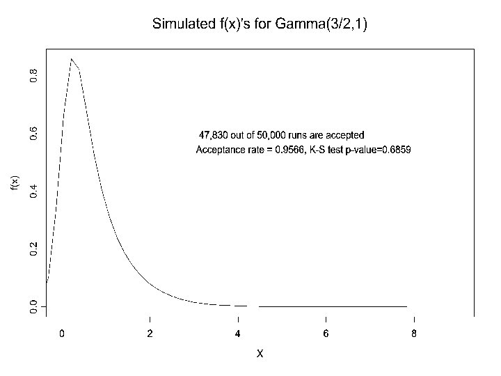
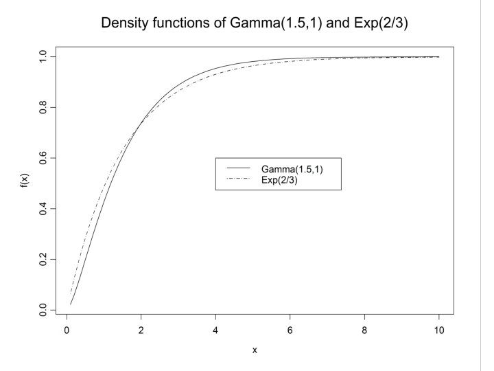
n Example 2. Generate Gamma(3/2, 1), i. e. We want to generate X from The max. of f(x)/g(x) is obtained when since

n Algorithm: 1. Generate U 1, U 2 ~ U(0, 1) Let Y = -3 log U 1 /2. 2. Return X = Y if n Question: Why do we choose Y ~ Exp(2/3)? Gamma(3/2, 1) and Exp(2/3) have the same variance!

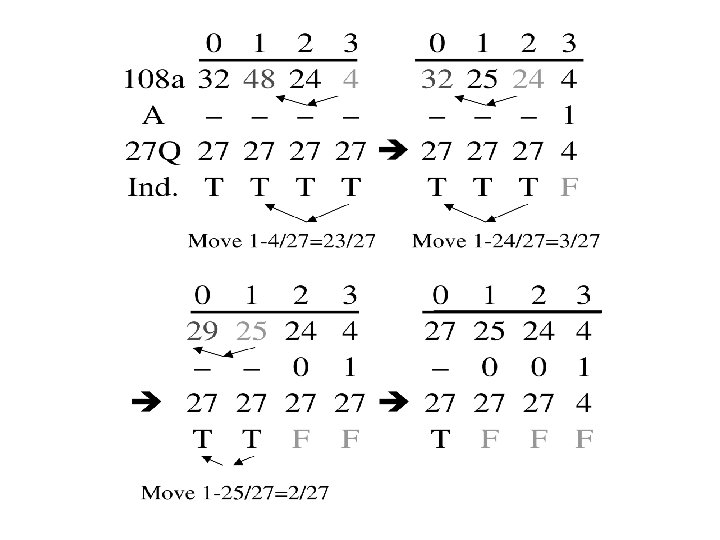
n Alias method: Looks like “rejection” but it is indeed “composition”. n Example 1. X ~ B(3, 1/3), i. e.

n Table method: (Composition) Example 1. X ~ B(3, 1/3) P(X=0)=0. 296 P(X=1)=0. 445 P(X=2)=0. 222 P(X=3)=0. 037 10 -1 10 -2 10 -3 2 9 6 4 4 5 2 2 2 0 3 7 8 18 20

n Algorithm: 1. Generate U ~ U(0, 1) 2. If 其中 a 1[. ] = 00 1111 22 a 2[. ] = 00000 1111 22 333 a 3[. ] = 00000 11111 22 3333333