N GREGORY MANKIW PRINCIPLES OF ECONOMICS Eighth Edition

N. GREGORY MANKIW PRINCIPLES OF ECONOMICS Eighth Edition CHAPTE R 13 The Costs of Production Premium Power. Point Slides by: V. Andreea CHIRITESCU Eastern Illinois University © 2018 Cengage Learning®. May not be scanned, copied or duplicated, or posted to a publicly accessible website, in whole or in part, except for use as permitted in a license distributed with a certain product or service or otherwise on a password-protected website or school-approved learning management system for classroom use. 1

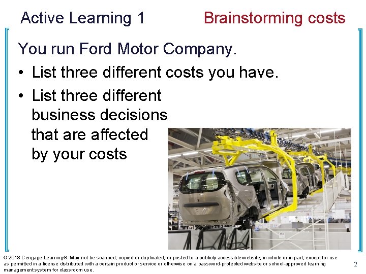
Active Learning 1 Brainstorming costs You run Ford Motor Company. • List three different costs you have. • List three different business decisions that are affected by your costs © 2018 Cengage Learning®. May not be scanned, copied or duplicated, or posted to a publicly accessible website, in whole or in part, except for use as permitted in a license distributed with a certain product or service or otherwise on a password-protected website or school-approved learning management system for classroom use. 2

Look for the answers to these questions: • What is a production function? What is marginal product? How are they related? • What are the various costs? How are they related to each other and to output? • How are costs different in the short run vs. the long run? • What are “economies of scale”? © 2018 Cengage Learning®. May not be scanned, copied or duplicated, or posted to a publicly accessible website, in whole or in part, except for use as permitted in a license distributed with a certain product or service or otherwise on a password-protected website or school-approved learning management system for classroom use. 3

Total Revenue, Total Cost, Profit • We assume that the firm’s goal is to maximize profit. Profit = Total revenue – Total cost the amount a firm receives from the sale of its output the market value of the inputs a firm uses in production TR = P×Q © 2018 Cengage Learning®. May not be scanned, copied or duplicated, or posted to a publicly accessible website, in whole or in part, except for use as permitted in a license distributed with a certain product or service or otherwise on a password-protected website or school-approved learning management system for classroom use. 4

Costs: Explicit vs. Implicit • ‘The cost of something is what you give up to get it. ’ • Explicit costs – Require an outlay of money • E. g. , paying wages to workers. • Implicit costs – Do not require a cash outlay • E. g. , the opportunity cost of the owner’s time. • Total cost = Explicit + Implicit costs © 2018 Cengage Learning®. May not be scanned, copied or duplicated, or posted to a publicly accessible website, in whole or in part, except for use as permitted in a license distributed with a certain product or service or otherwise on a password-protected website or school-approved learning management system for classroom use. 5

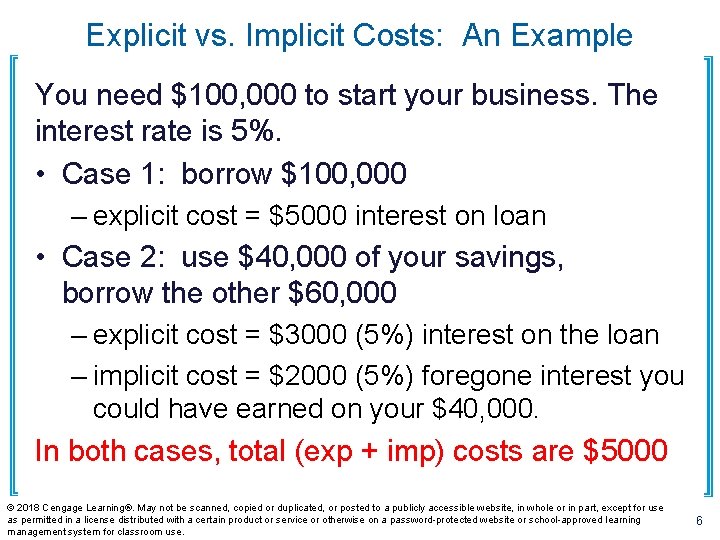
Explicit vs. Implicit Costs: An Example You need $100, 000 to start your business. The interest rate is 5%. • Case 1: borrow $100, 000 – explicit cost = $5000 interest on loan • Case 2: use $40, 000 of your savings, borrow the other $60, 000 – explicit cost = $3000 (5%) interest on the loan – implicit cost = $2000 (5%) foregone interest you could have earned on your $40, 000. In both cases, total (exp + imp) costs are $5000 © 2018 Cengage Learning®. May not be scanned, copied or duplicated, or posted to a publicly accessible website, in whole or in part, except for use as permitted in a license distributed with a certain product or service or otherwise on a password-protected website or school-approved learning management system for classroom use. 6

Economic Profit vs. Accounting Profit • Accounting profit =total revenue minus total explicit costs • Economic profit =total revenue minus total costs (including explicit and implicit costs) • Accounting profit ignores implicit costs, so it’s higher than economic profit. © 2018 Cengage Learning®. May not be scanned, copied or duplicated, or posted to a publicly accessible website, in whole or in part, except for use as permitted in a license distributed with a certain product or service or otherwise on a password-protected website or school-approved learning management system for classroom use. 7

Active Learning 2 Economic profit vs. accounting profit The equilibrium rent on office space has just increased by $500/month. Determine the effects on accounting profit and economic profit if: a. you rent your office space b. you own your office space © 2018 Cengage Learning®. May not be scanned, copied or duplicated, or posted to a publicly accessible website, in whole or in part, except for use as permitted in a license distributed with a certain product or service or otherwise on a password-protected website or school-approved learning management system for classroom use. 8

Active Learning 2 Answers The rent on office space increases $500/month. a. You rent your office space. • Explicit costs increase $500/month. Accounting profit & economic profit each fall $500/month. b. You own your office space. • Explicit costs do not change, so accounting profit does not change. • Implicit costs increase $500/month (opp. cost of using your space instead of renting it) so economic profit falls by $500/month. © 2018 Cengage Learning®. May not be scanned, copied or duplicated, or posted to a publicly accessible website, in whole or in part, except for use as permitted in a license distributed with a certain product or service or otherwise on a password-protected website or school-approved learning management system for classroom use. 9

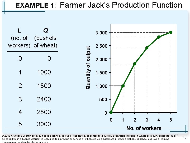
Production Function • Production function – Relationship between • Quantity of inputs used to make a good • And the quantity of output of that good – Gets flatter as production rises © 2018 Cengage Learning®. May not be scanned, copied or duplicated, or posted to a publicly accessible website, in whole or in part, except for use as permitted in a license distributed with a certain product or service or otherwise on a password-protected website or school-approved learning management system for classroom use. 10

EXAMPLE 1: Farmer Jack Example 1: • Farmer Jack grows wheat. • He has 5 acres of land (fixed resource). • He can hire as many workers as he wants. – The quantity of output produced varies with the number of workers hired © 2018 Cengage Learning®. May not be scanned, copied or duplicated, or posted to a publicly accessible website, in whole or in part, except for use as permitted in a license distributed with a certain product or service or otherwise on a password-protected website or school-approved learning management system for classroom use. 11

EXAMPLE 1: Farmer Jack’s Production Function Q (no. of (bushels workers) of wheat) 3, 000 Quantity of output L 2, 500 0 0 1 1000 2 1800 3 2400 500 4 2800 0 5 3000 2, 000 1, 500 1, 000 0 1 2 3 4 5 No. of workers 12 © 2018 Cengage Learning®. May not be scanned, copied or duplicated, or posted to a publicly accessible website, in whole or in part, except for use as permitted in a license distributed with a certain product or service or otherwise on a password-protected website or school-approved learning 12

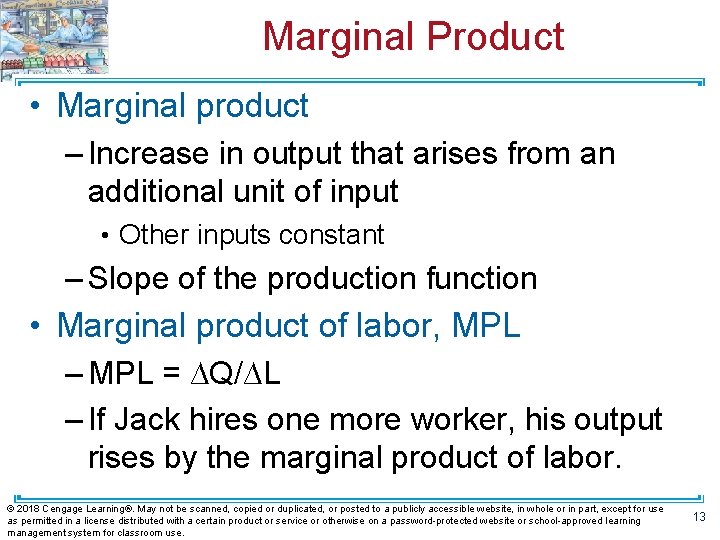
Marginal Product • Marginal product – Increase in output that arises from an additional unit of input • Other inputs constant – Slope of the production function • Marginal product of labor, MPL – MPL = ∆Q/∆L – If Jack hires one more worker, his output rises by the marginal product of labor. © 2018 Cengage Learning®. May not be scanned, copied or duplicated, or posted to a publicly accessible website, in whole or in part, except for use as permitted in a license distributed with a certain product or service or otherwise on a password-protected website or school-approved learning management system for classroom use. 13

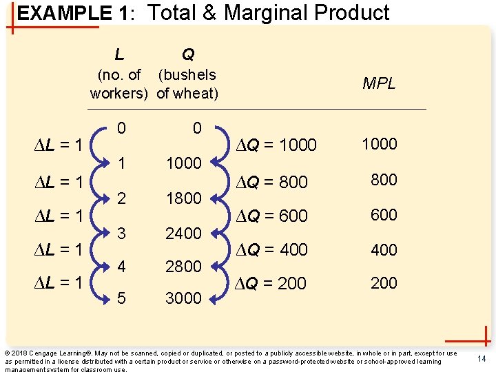
EXAMPLE 1: Total & Marginal Product L Q (no. of (bushels workers) of wheat) ∆L = 1 ∆L = 1 0 0 1 1000 2 1800 3 2400 4 2800 5 3000 MPL ∆Q = 1000 ∆Q = 800 ∆Q = 600 ∆Q = 400 ∆Q = 200 © 2018 Cengage Learning®. May not be scanned, copied or duplicated, or posted to a publicly accessible website, in whole or in part, except for use as permitted in a license distributed with a certain product or service or otherwise on a password-protected website or school-approved learning management system for classroom use. 14

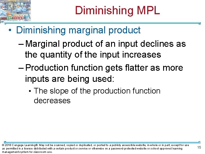
Diminishing MPL • Diminishing marginal product – Marginal product of an input declines as the quantity of the input increases – Production function gets flatter as more inputs are being used: • The slope of the production function decreases © 2018 Cengage Learning®. May not be scanned, copied or duplicated, or posted to a publicly accessible website, in whole or in part, except for use as permitted in a license distributed with a certain product or service or otherwise on a password-protected website or school-approved learning management system for classroom use. 15

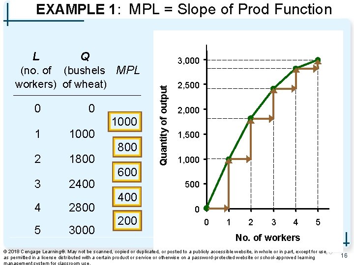
EXAMPLE 1: MPL = Slope of Prod Function Q (no. of (bushels MPL workers) of wheat) 0 1 2 3 4 5 0 1000 1800 2400 2800 3000 1000 800 600 400 200 3, 000 MPL Quantity of output L equals the slope of the 2, 500 production function. 2, 000 Notice that MPL diminishes 1, 500 as L increases. 1, 000 This explains why 500 production the function gets flatter 0 as L 0 increases. 1 2 3 4 5 No. of workers 16 © 2018 Cengage Learning®. May not be scanned, copied or duplicated, or posted to a publicly accessible website, in whole or in part, except for use as permitted in a license distributed with a certain product or service or otherwise on a password-protected website or school-approved learning 16

Why MPL Is Important • ‘Rational people think at the margin’ • When Farmer Jack hires an extra worker – His costs rise by the wage he pays the worker – His output rises by MPL – Comparing them helps Jack decide whether he should hire the worker. © 2018 Cengage Learning®. May not be scanned, copied or duplicated, or posted to a publicly accessible website, in whole or in part, except for use as permitted in a license distributed with a certain product or service or otherwise on a password-protected website or school-approved learning management system for classroom use. 17

Why MPL Diminishes • Farmer Jack’s output rises by a smaller and smaller amount for each additional worker. Why? – As Jack adds workers, the average worker has less land to work with and will be less productive. – In general, MPL diminishes as L rises whether the fixed input is land or capital (equipment, machines, etc. ). © 2018 Cengage Learning®. May not be scanned, copied or duplicated, or posted to a publicly accessible website, in whole or in part, except for use as permitted in a license distributed with a certain product or service or otherwise on a password-protected website or school-approved learning management system for classroom use. 18

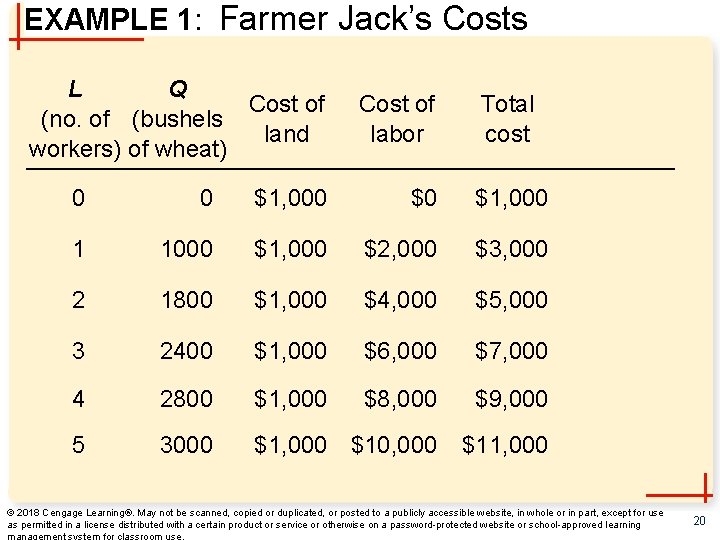
EXAMPLE 1: Farmer Jack’s Costs Farmer Jack must pay $1000 per month for the land, regardless of how much wheat he grows. The market wage for a farm worker is $2000 per month. • So Farmer Jack’s costs are related to how much wheat he produces…. © 2018 Cengage Learning®. May not be scanned, copied or duplicated, or posted to a publicly accessible website, in whole or in part, except for use as permitted in a license distributed with a certain product or service or otherwise on a password-protected website or school-approved learning management system for classroom use. 19

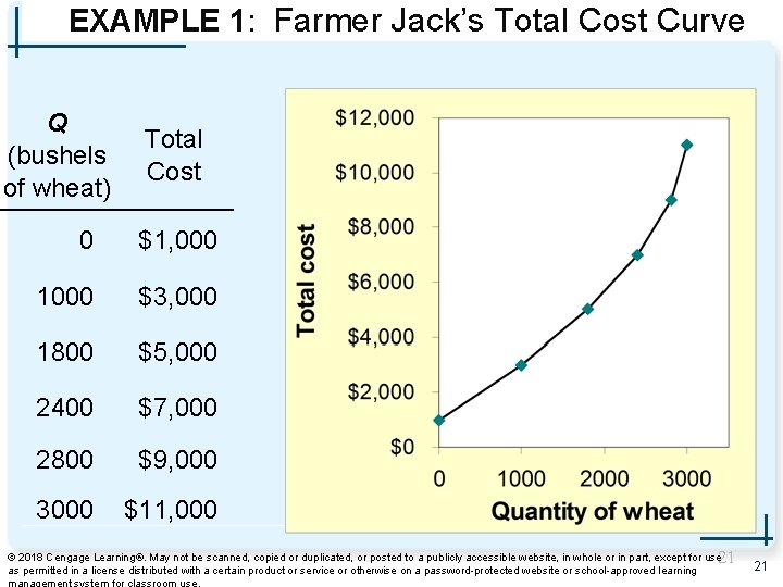
EXAMPLE 1: Farmer Jack’s Costs L Q Cost of (no. of (bushels land workers) of wheat) Cost of labor Total cost 0 0 $1, 000 $0 $1, 000 1 1000 $1, 000 $2, 000 $3, 000 2 1800 $1, 000 $4, 000 $5, 000 3 2400 $1, 000 $6, 000 $7, 000 4 2800 $1, 000 $8, 000 $9, 000 5 3000 $1, 000 $10, 000 $11, 000 © 2018 Cengage Learning®. May not be scanned, copied or duplicated, or posted to a publicly accessible website, in whole or in part, except for use as permitted in a license distributed with a certain product or service or otherwise on a password-protected website or school-approved learning management system for classroom use. 20

EXAMPLE 1: Farmer Jack’s Total Cost Curve Q (bushels of wheat) Total Cost 0 $1, 000 1000 $3, 000 1800 $5, 000 2400 $7, 000 2800 $9, 000 3000 $11, 000 21 © 2018 Cengage Learning®. May not be scanned, copied or duplicated, or posted to a publicly accessible website, in whole or in part, except for use as permitted in a license distributed with a certain product or service or otherwise on a password-protected website or school-approved learning 21

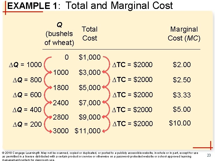
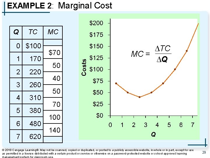
Marginal Cost • Marginal cost, MC – Increase in total cost arising from an extra unit of production – Marginal cost = Change in total cost / Change in quantity – MC = ΔTC / ΔQ – Increase in total cost • From producing an additional unit of output © 2018 Cengage Learning®. May not be scanned, copied or duplicated, or posted to a publicly accessible website, in whole or in part, except for use as permitted in a license distributed with a certain product or service or otherwise on a password-protected website or school-approved learning management system for classroom use. 22

EXAMPLE 1: Total and Marginal Cost Q (bushels of wheat) ∆Q = 1000 ∆Q = 800 ∆Q = 600 ∆Q = 400 ∆Q = 200 Marginal Cost (MC) Total Cost 0 $1, 000 1000 $3, 000 1800 $5, 000 2400 $7, 000 2800 $9, 000 3000 $11, 000 ∆TC = $2000 $2. 50 ∆TC = $2000 $3. 33 ∆TC = $2000 $5. 00 ∆TC = $2000 $10. 00 © 2018 Cengage Learning®. May not be scanned, copied or duplicated, or posted to a publicly accessible website, in whole or in part, except for use as permitted in a license distributed with a certain product or service or otherwise on a password-protected website or school-approved learning management system for classroom use. 23

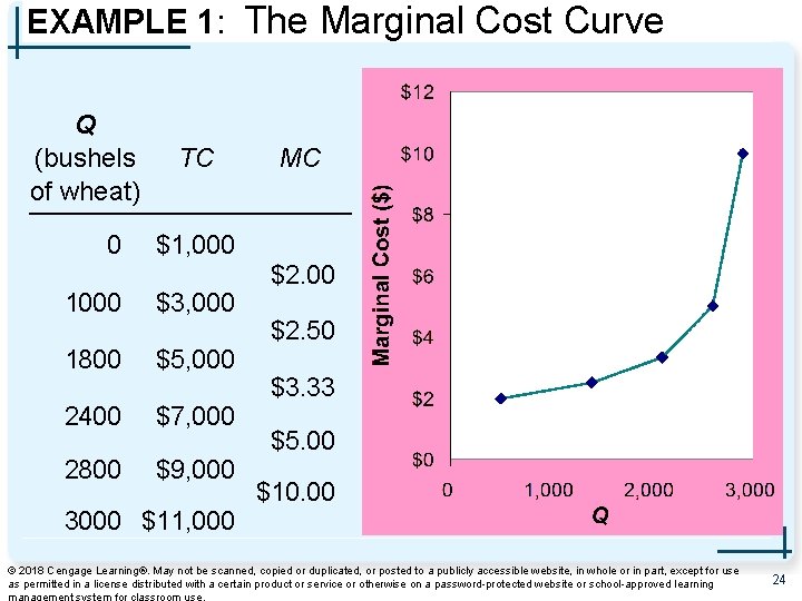
EXAMPLE 1: The Marginal Cost Curve Q (bushels of wheat) 0 TC MC $1, 000 1000 $3, 000 1800 $5, 000 2400 $7, 000 2800 $9, 000 3000 $11, 000 MC usually rises as Q rises, as in this example. $2. 00 $2. 50 $3. 33 $5. 00 $10. 00 © 2018 Cengage Learning®. May not be scanned, copied or duplicated, or posted to a publicly accessible website, in whole or in part, except for use as permitted in a license distributed with a certain product or service or otherwise on a password-protected website or school-approved learning 24

Why MC Is Important • Farmer Jack is rational and wants to maximize his profit – To increase profit, should he produce more or less wheat? • Farmer Jack needs to “think at the margin” – If the cost of additional wheat (MC) is less than the revenue he would get from selling it, then Jack’s profits rise if he produces more. © 2018 Cengage Learning®. May not be scanned, copied or duplicated, or posted to a publicly accessible website, in whole or in part, except for use as permitted in a license distributed with a certain product or service or otherwise on a password-protected website or school-approved learning management system for classroom use. 25

Fixed and Variable Costs • Fixed costs, FC, do not vary with the quantity of output produced – For Farmer Jack, FC = $1000 for his land – Other examples: cost of equipment, loan payments, rent • Variable costs, VC, vary with the quantity of output produced • For Farmer Jack, VC = wages he pays workers • Other example: cost of materials • Total cost = Fixed cost + Variable cost © 2018 Cengage Learning®. May not be scanned, copied or duplicated, or posted to a publicly accessible website, in whole or in part, except for use as permitted in a license distributed with a certain product or service or otherwise on a password-protected website or school-approved learning management system for classroom use. 26

EXAMPLE 2: Production Costs • Our second example is more general, applies to any type of firm producing any good with any types of inputs. – Calculate and graph TC knowing FC and VC – Calculate and graph marginal and average costs – Understand the relationship between marginal cost and average cost © 2018 Cengage Learning®. May not be scanned, copied or duplicated, or posted to a publicly accessible website, in whole or in part, except for use as permitted in a license distributed with a certain product or service or otherwise on a password-protected website or school-approved learning management system for classroom use. 27

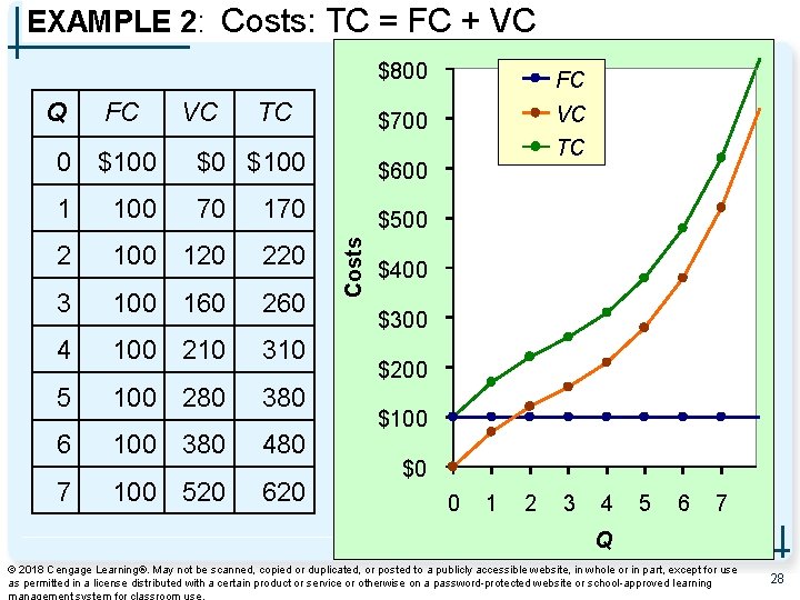
EXAMPLE 2: Costs: TC = FC + VC Q FC VC TC $800 FC $700 VC $0 $100 $600 1 100 70 170 $500 2 100 120 220 3 100 160 260 4 100 210 310 5 100 280 380 6 100 380 480 7 100 520 620 Costs 0 $100 TC $400 $300 $200 $100 $0 0 1 2 3 4 5 6 7 Q © 2018 Cengage Learning®. May not be scanned, copied or duplicated, or posted to a publicly accessible website, in whole or in part, except for use as permitted in a license distributed with a certain product or service or otherwise on a password-protected website or school-approved learning 28

EXAMPLE 2: Marginal Cost Q TC 0 $100 1 170 2 220 3 260 4 310 5 380 6 480 7 620 MC $70 50 40 50 70 100 140 Recall, Marginal Cost (MC) is the change in total cost from producing one more unit: ∆TC MC = ∆Q Usually, MC rises as Q rises, due to diminishing marginal product. Sometimes (as here), MC falls before rising. (In other examples, MC may be constant. ) © 2018 Cengage Learning®. May not be scanned, copied or duplicated, or posted to a publicly accessible website, in whole or in part, except for use as permitted in a license distributed with a certain product or service or otherwise on a password-protected website or school-approved learning 29

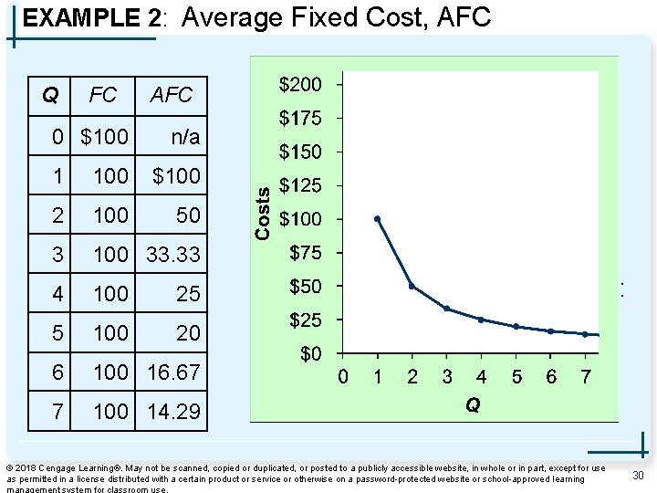
EXAMPLE 2: Average Fixed Cost, AFC Q FC 0 $100 AFC n/a 1 100 $100 2 100 50 3 100 33. 33 4 100 25 5 100 20 6 100 16. 67 7 100 14. 29 Average fixed cost (AFC) is fixed cost divided by the quantity of output: AFC = FC/Q Notice that AFC falls as Q rises: The firm is spreading its fixed costs over a larger and larger number of units. © 2018 Cengage Learning®. May not be scanned, copied or duplicated, or posted to a publicly accessible website, in whole or in part, except for use as permitted in a license distributed with a certain product or service or otherwise on a password-protected website or school-approved learning 30

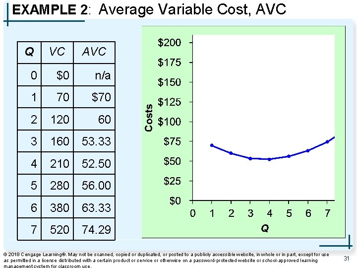
EXAMPLE 2: Average Variable Cost, AVC Q VC AVC 0 $0 n/a 1 70 $70 2 120 60 3 160 53. 33 4 210 52. 50 5 280 56. 00 6 380 63. 33 7 520 74. 29 Average variable cost (AVC) is variable cost divided by the quantity of output: AVC = VC/Q As Q rises, AVC may fall initially. In most cases, AVC will eventually rise as output rises. © 2018 Cengage Learning®. May not be scanned, copied or duplicated, or posted to a publicly accessible website, in whole or in part, except for use as permitted in a license distributed with a certain product or service or otherwise on a password-protected website or school-approved learning 31

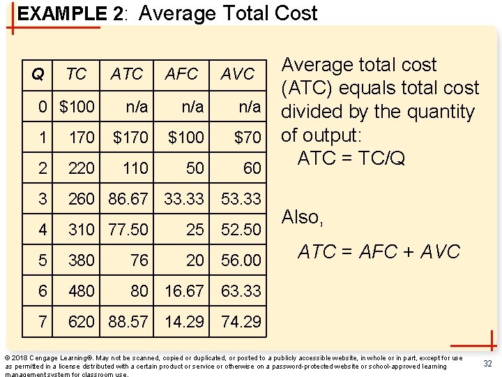
EXAMPLE 2: Average Total Cost Q TC 0 $100 ATC AFC AVC n/a n/a 1 170 $100 $70 2 220 110 50 60 3 260 86. 67 33. 33 53. 33 4 310 77. 50 25 52. 50 5 380 76 20 56. 00 6 480 80 16. 67 63. 33 7 620 88. 57 14. 29 74. 29 Average total cost (ATC) equals total cost divided by the quantity of output: ATC = TC/Q Also, ATC = AFC + AVC © 2018 Cengage Learning®. May not be scanned, copied or duplicated, or posted to a publicly accessible website, in whole or in part, except for use as permitted in a license distributed with a certain product or service or otherwise on a password-protected website or school-approved learning management system for classroom use. 32

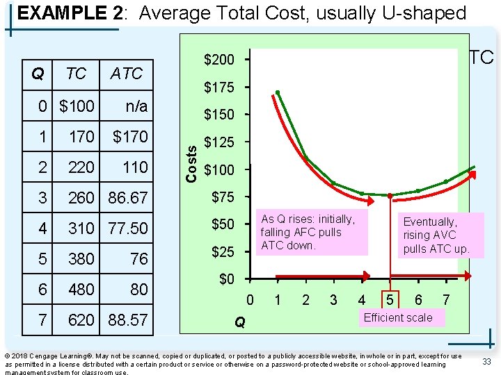
EXAMPLE 2: Average Total Cost, usually U-shaped Q TC 0 $100 ATC Usually, as in this example, the ATC $200 curve $175 is U-shaped. n/a $150 170 $170 2 220 110 3 260 86. 67 $75 4 310 77. 50 $50 5 380 76 6 480 80 7 620 88. 57 Costs 1 $125 $100 As Q rises: initially, falling AFC pulls ATC down. Eventually, rising AVC pulls ATC up. Efficient scale: $25 The quantity that minimizes ATC. $0 0 Q 1 2 3 4 5 6 7 Efficient scale © 2018 Cengage Learning®. May not be scanned, copied or duplicated, or posted to a publicly accessible website, in whole or in part, except for use as permitted in a license distributed with a certain product or service or otherwise on a password-protected website or school-approved learning 33

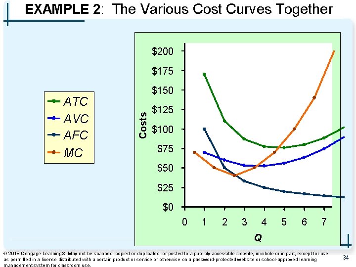
EXAMPLE 2: The Various Cost Curves Together $200 $175 Costs ATC AVC AFC MC $150 $125 $100 $75 $50 $25 $0 0 1 2 3 4 5 6 7 Q © 2018 Cengage Learning®. May not be scanned, copied or duplicated, or posted to a publicly accessible website, in whole or in part, except for use as permitted in a license distributed with a certain product or service or otherwise on a password-protected website or school-approved learning 34

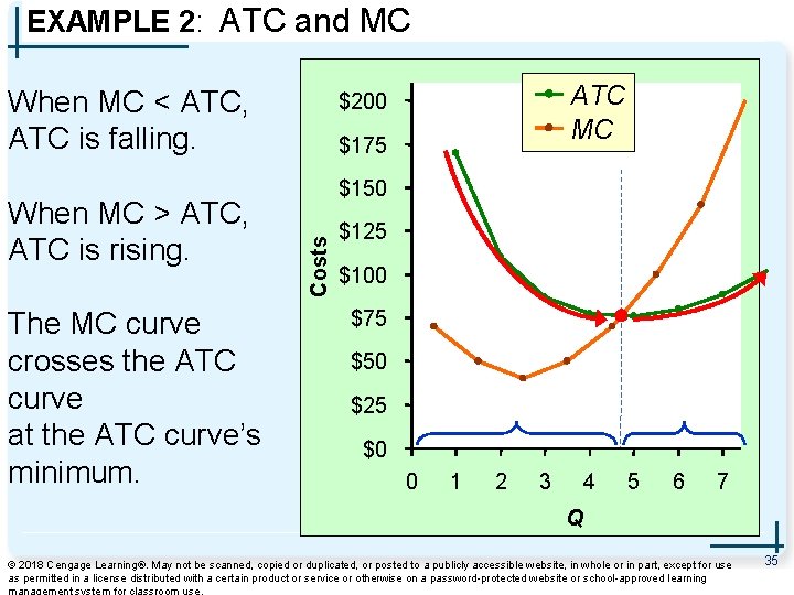
EXAMPLE 2: ATC and MC When MC < ATC, ATC is falling. The MC curve crosses the ATC curve at the ATC curve’s minimum. $175 $150 Costs When MC > ATC, ATC is rising. ATC MC $200 $125 $100 $75 $50 $25 $0 0 1 2 3 4 5 6 7 Q © 2018 Cengage Learning®. May not be scanned, copied or duplicated, or posted to a publicly accessible website, in whole or in part, except for use as permitted in a license distributed with a certain product or service or otherwise on a password-protected website or school-approved learning 35

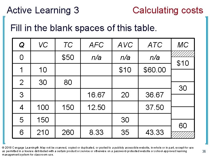
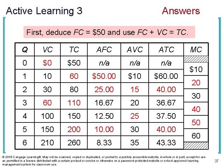
Active Learning 3 Calculating costs Fill in the blank spaces of this table. Q VC 0 1 10 2 30 TC AFC AVC ATC $50 n/a n/a $10 $60. 00 80 3 16. 67 4 100 5 150 6 210 150 20 12. 50 36. 67 8. 33 $10 30 37. 50 30 260 MC 35 43. 33 60 © 2018 Cengage Learning®. May not be scanned, copied or duplicated, or posted to a publicly accessible website, in whole or in part, except for use as permitted in a license distributed with a certain product or service or otherwise on a password-protected website or school-approved learning management system for classroom use. 36

Active Learning 3 Answers Use AFC ATC AVC == FC/Q TC/Q VC/Q MC and First, relationship deduce FC between = $50 and use FCTC + VC = TC. Q VC TC AFC AVC ATC 0 $0 $50 n/a n/a 1 10 60 $50. 00 $10 $60. 00 2 30 80 25. 00 15 40. 00 3 60 110 16. 67 20 36. 67 4 100 150 12. 50 25 37. 50 5 150 200 10. 00 30 40. 00 6 210 260 8. 33 35 43. 33 MC $10 20 30 40 50 60 © 2018 Cengage Learning®. May not be scanned, copied or duplicated, or posted to a publicly accessible website, in whole or in part, except for use as permitted in a license distributed with a certain product or service or otherwise on a password-protected website or school-approved learning management system for classroom use. 37

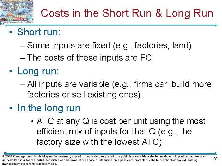
Costs in the Short Run & Long Run • Short run: – Some inputs are fixed (e. g. , factories, land) – The costs of these inputs are FC • Long run: – All inputs are variable (e. g. , firms can build more factories or sell existing ones) • In the long run • ATC at any Q is cost per unit using the most efficient mix of inputs for that Q (e. g. , the factory size with the lowest ATC) © 2018 Cengage Learning®. May not be scanned, copied or duplicated, or posted to a publicly accessible website, in whole or in part, except for use as permitted in a license distributed with a certain product or service or otherwise on a password-protected website or school-approved learning management system for classroom use. 38

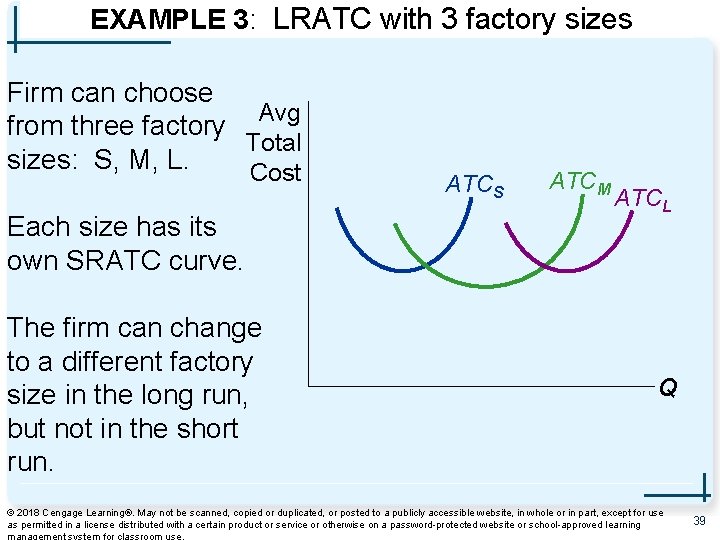
EXAMPLE 3: LRATC with 3 factory sizes Firm can choose Avg from three factory Total sizes: S, M, L. Cost Each size has its own SRATC curve. The firm can change to a different factory size in the long run, but not in the short run. ATCS ATCM ATCL Q © 2018 Cengage Learning®. May not be scanned, copied or duplicated, or posted to a publicly accessible website, in whole or in part, except for use as permitted in a license distributed with a certain product or service or otherwise on a password-protected website or school-approved learning 39

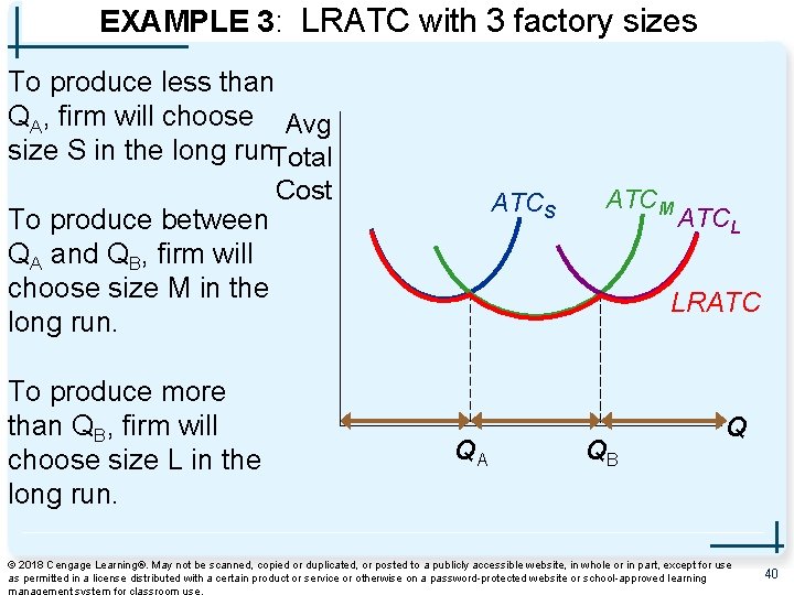
EXAMPLE 3: LRATC with 3 factory sizes To produce less than QA, firm will choose Avg size S in the long run. Total Cost To produce between QA and QB, firm will choose size M in the long run. To produce more than QB, firm will choose size L in the long run. ATCS ATCM ATCL LRATC QA QB Q © 2018 Cengage Learning®. May not be scanned, copied or duplicated, or posted to a publicly accessible website, in whole or in part, except for use as permitted in a license distributed with a certain product or service or otherwise on a password-protected website or school-approved learning 40

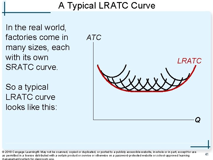
A Typical LRATC Curve In the real world, factories come in many sizes, each with its own SRATC curve. ATC LRATC So a typical LRATC curve looks like this: Q © 2018 Cengage Learning®. May not be scanned, copied or duplicated, or posted to a publicly accessible website, in whole or in part, except for use as permitted in a license distributed with a certain product or service or otherwise on a password-protected website or school-approved learning 41

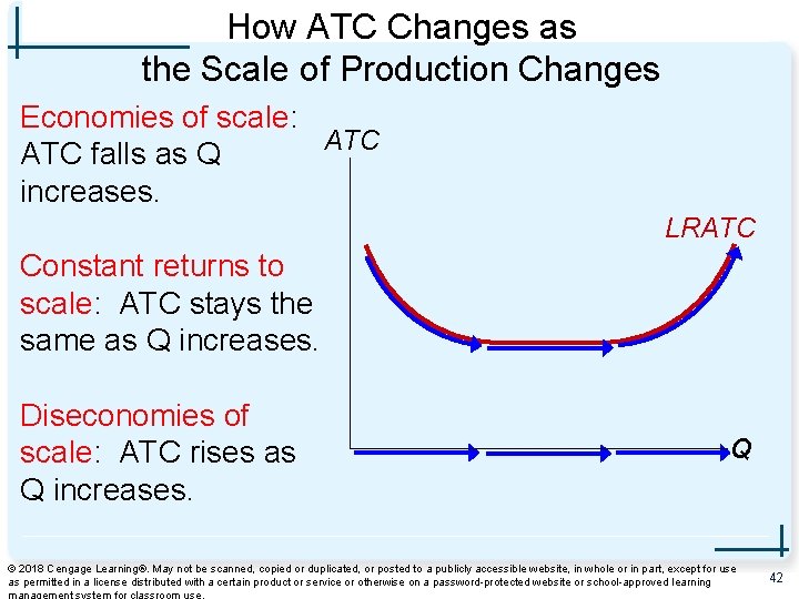
How ATC Changes as the Scale of Production Changes Economies of scale: ATC falls as Q increases. LRATC Constant returns to scale: ATC stays the same as Q increases. Diseconomies of scale: ATC rises as Q increases. Q © 2018 Cengage Learning®. May not be scanned, copied or duplicated, or posted to a publicly accessible website, in whole or in part, except for use as permitted in a license distributed with a certain product or service or otherwise on a password-protected website or school-approved learning 42

Costs in Short and Long Run • Economies of scale – Long-run average total cost falls as the quantity of output increases • Increasing specialization among workers • More common when Q is low • Constant returns to scale – Long-run average total cost stays the same as the quantity of output changes © 2018 Cengage Learning®. May not be scanned, copied or duplicated, or posted to a publicly accessible website, in whole or in part, except for use as permitted in a license distributed with a certain product or service or otherwise on a password-protected website or school-approved learning management system for classroom use. 43

Costs in Short and Long Run • Diseconomies of scale – Long-run average total cost rises as the quantity of output increases – Increasing coordination problems in large organizations. • E. g. , management becomes stretched, can’t control costs. • More common when Q is high. © 2018 Cengage Learning®. May not be scanned, copied or duplicated, or posted to a publicly accessible website, in whole or in part, except for use as permitted in a license distributed with a certain product or service or otherwise on a password-protected website or school-approved learning management system for classroom use. 44

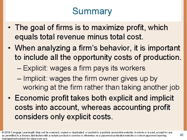
Summary • The goal of firms is to maximize profit, which equals total revenue minus total cost. • When analyzing a firm’s behavior, it is important to include all the opportunity costs of production. – Explicit: wages a firm pays its workers – Implicit: wages the firm owner gives up by working at the firm rather than taking another job • Economic profit takes both explicit and implicit costs into account, whereas accounting profit considers only explicit costs. © 2018 Cengage Learning®. May not be scanned, copied or duplicated, or posted to a publicly accessible website, in whole or in part, except for use as permitted in a license distributed with a certain product or service or otherwise on a password-protected website or school-approved learning management system for classroom use. 45

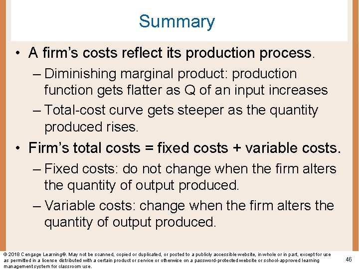
Summary • A firm’s costs reflect its production process. – Diminishing marginal product: production function gets flatter as Q of an input increases – Total-cost curve gets steeper as the quantity produced rises. • Firm’s total costs = fixed costs + variable costs. – Fixed costs: do not change when the firm alters the quantity of output produced. – Variable costs: change when the firm alters the quantity of output produced. © 2018 Cengage Learning®. May not be scanned, copied or duplicated, or posted to a publicly accessible website, in whole or in part, except for use as permitted in a license distributed with a certain product or service or otherwise on a password-protected website or school-approved learning management system for classroom use. 46

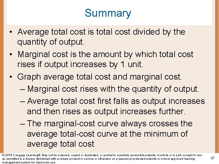
Summary • Average total cost is total cost divided by the quantity of output. • Marginal cost is the amount by which total cost rises if output increases by 1 unit. • Graph average total cost and marginal cost. – Marginal cost rises with the quantity of output. – Average total cost first falls as output increases and then rises as output increases further. – The marginal-cost curve always crosses the average total-cost curve at the minimum of average total cost © 2018 Cengage Learning®. May not be scanned, copied or duplicated, or posted to a publicly accessible website, in whole or in part, except for use as permitted in a license distributed with a certain product or service or otherwise on a password-protected website or school-approved learning management system for classroom use. 47

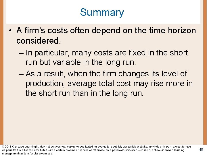
Summary • A firm’s costs often depend on the time horizon considered. – In particular, many costs are fixed in the short run but variable in the long run. – As a result, when the firm changes its level of production, average total cost may rise more in the short run than in the long run. © 2018 Cengage Learning®. May not be scanned, copied or duplicated, or posted to a publicly accessible website, in whole or in part, except for use as permitted in a license distributed with a certain product or service or otherwise on a password-protected website or school-approved learning management system for classroom use. 48