N B the material derivative rate of change

N. B. the ‘material derivative’, rate of change following the motion:

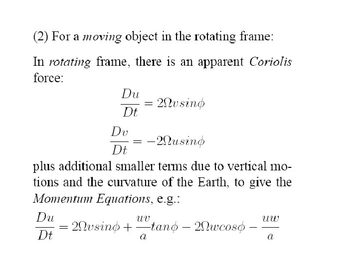
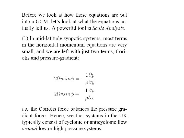
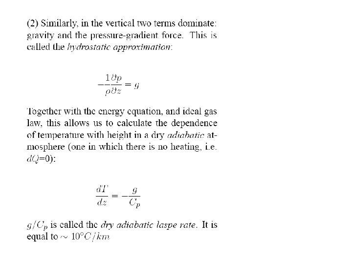
Approximations to full equations for use in a GCM 1. r = a + z (a=radius of Earth) z << a 2. Coriolis and metric terms proportional to can be ignored 3. For large scales, vertical acceleration is small, hence vertical component becomes:

“Primitive Equations”

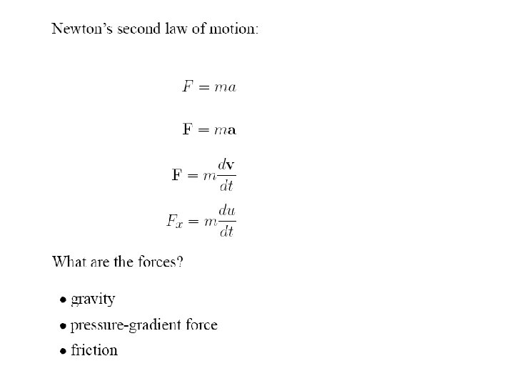
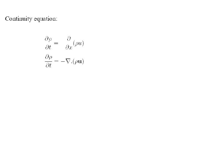
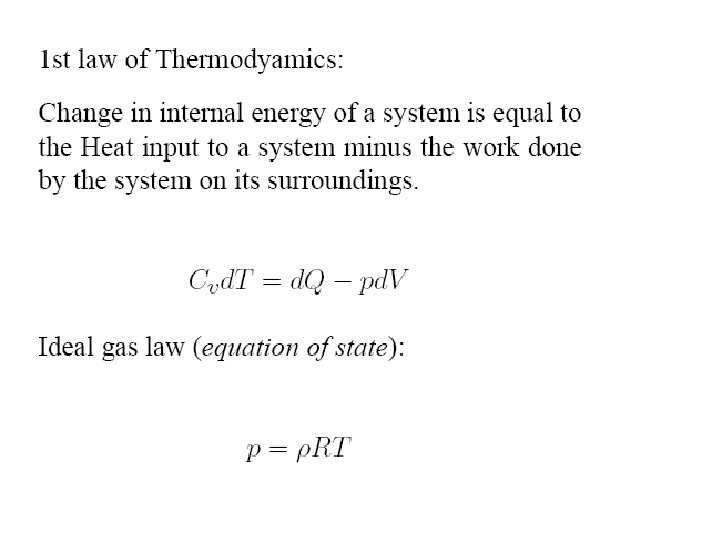
Plus other equations • Continuity equation • Ideal Gas Law • First Law of Thermodynamics These equations can be shown to conserve energy, angular momentum, and mass.

How to solve equations? • Few analytical solutions to full Navier-Stokes equations, and only for fairly idealised problems. Hence need to solve numerically. • At heart of all numerical schemes is a Taylor series expansion: – Suppose we have an interval L, covered by N equally spaced grid points, xj=(j-1) Δx, then

Re-arrange to give approximation for derivatives • First order accurate: • Second order accurate • Fourth order accurate

Linear Advection Equation Differential equation becomes following difference equation Second order accurate in both space and time Centered time and space scheme

Numerical Stability and numerical solutions • Schemes may be accurate but unstable: – e. g. simple centred difference scheme for linear advection scheme will be stable only if Courant. Friedrichs-Levy number less than 1. • Many schemes can have artificial (computational mode) • All schemes distort true solution (e. g. change phase and/or group speed) • Some schemes fail to conserve properties of system (e. g. energy)

Examples of Numerical Schemes