MXG Tools and Usage Chuck Hopf PPT Available

MXG Tools and Usage Chuck Hopf PPT Available at MXG. COM Download Site

Agenda – Building the PDB • • Installing MXG z. OS and ASCII Tailoring MXG UTILWORK VMXGALOCVGETALOC UTILBLDP BLDSMPDB READDB 2 VMXGSUM

Agenda - Analysis • • ANALID ANALGRID ANALCOMP VMXGPRNT VMXGFIND VMXGSRCH ANALCNCR ANALCAPD

Installing MXG – z. OS • Download either the TRSversion. TRS or the EBCversion. EBC datasets from the MXG website. TRS is a tersed copy of the MXG SOURCLIB and when untersed creates the PDS containing all of the SOURCE. The EBC version is in IEBUPDTE format and requires you to run IEBUPDTE to create the SOURCLIB. Either will work – it is a matter of which you find easier.

Installing MXG – z. OS • FTP Tersed – – – – //FTPMXG EXEC PGM=FTP, PARM='(EXIT=4' //SYSPRINT DD SYSOUT=*, DCB=BLKSIZE=133 //SYSABEND DD SYSOUT=* //SYSOUT DD SYSOUT=* //FTPOUT DD SYSOUT=* //SYSIN DD * 70. 86. 188. 234 USERID PASSWORD LOCSITE LRECL=1024 RECFM=FB BLKSIZE=6144 LOCSITe u. NIT=SYSDA PRIMARY=5000 SECONDARY=300 BINARY GET TER 3006. TER 'MXG. TER 3006. TER' (REPLACE CLOSE QUIT

Installing MXG - z. OS • FTP IEBUPDTE //FTPMXG EXEC PGM=FTP, PARM='(EXIT=4' //SYSPRINT DD SYSOUT=*, DCB=BLKSIZE=133 //SYSABEND DD SYSOUT=* //SYSOUT DD SYSOUT=* //FTPOUT DD SYSOUT=* //SYSIN DD * 70. 86. 188. 234 USERID PASSWORD LOCSITE LRECL=80 RECFM=FB BLKSIZE=0 LOCSITE UNIT=SYSDA PRIMARY=5000 SECONDARY=300 GET EBC 3006. EBC 'MXG. V 3006. EBCDIC’ (REPLACE CLOSE QUIT

Installing MXG - z. OS • UNTERSE //UNTERSE EXEC PGM=TRSMAIN, PARM='UNPACK' //SYSPRINT DD SYSOUT=* //INFILE DD DSN=MXG. TER 3006. TER, DISP=SHR //OUTFILE DD DSN=MXG. V 3006. MXG. SOURCLIB, UNIT=SYSDA, // DISP=(NEW, CATLG), RECFM=FB, LRECL=80, BLKSIZE=0, // AVGREC=M, SPACE=(80, (3, 1, 1199)) PDS: 3 MIL 80 BYTE RECS

Installing MXG - z. OS • IEBUPDTE //STEP 1 EXEC PGM=IEBUPDTE, PARM=NEW //SYSPRINT DD DUMMY PRINTS 3, 000+ LINES, THE ENTIRE MXG //* SOURCE LIBRARY, IF UN-DUMMIED; DON'T DOIT. //SYSIN DD DSN=MXG. V 3006. EBCDIC, DISP=SHR //SYSUT 2 DD DSN=MXG. V 3006. MXG. SOURCLIB, UNIT=SYSDA, // DISP=(NEW, CATLG), RECFM=FB, LRECL=80, BLKSIZE=0, // AVGREC=M, SPACE=(80, (3, 1, 1199)) PDS: 3 MIL 80 BYTE RECS

Installing MXG - z. OS • Building one or more USERID. SOURCLIBs. • Why more than one? ? – Sometimes putting in an entire new release is not necessary but it can result in mounds of paperwork (which we all love. ) – Putting in a single member can reduce the paperwork since it then becomes a ‘fix’ and not a new release – Putting those ‘fixes’ into a CHANGES. SOURCLIB between new releases and then emptying CHANGES when you put in the new release can be simpler

Installing MXG – z. OS • Building USER SOURCLIBs //STEP 2 EXEC PGM=IEFBR 14 //USERID DD DSN=MXG. USERID. SOURCLIB, UNIT=SYSDA, // DISP=(NEW, CATLG), RECFM=FB, LRECL=80, BLKSIZE=0, // SPACE=(CYL, (15, 99)) //CHANGES DD DSN=MXG. CHANGES. SOURCLIB, UNIT=SYSDA, // DISP=(NEW, CATLG), RECFM=FB, LRECL=80, BLKSIZE=0, // SPACE=(CYL, (15, 99))

Installing MXG - z. OS • Run FORMATS //FORMATS EXEC SAS, ENTRY=SAS, // CONFIG='MXG. V 3006. MXG. SOURCLIB(CONFIGV 9)' //SASLOG DD SYSOUT=* //SASLIST DD SYSOUT=* //SOURCLIB DD DSN=MXG. USERID. SOURCLIB, DISP=SHR // DD DSN=MXG. CHANGES. SOURCLIB, DISP=SHR // DD DSN=MXG. V 3006. MXG. SOURCLIB, DISP=SHR //LIBRARY DD DSN=MXG. V 3006. MXG. FORMATS, // UNIT=SYSDA, DISP=(NEW, CATLG), SPACE=(CYL, (12, 2)) //SYSIN DD * %INCLUDE SOURCLIB(FORMATS); //*

Installing MXG - z. OS • An MXGSAS PROC is no longer required. • In your USERID. SOURCLIB create a member MXGNAMES as follows: %LET MXGSOURC=MXG. V 3006. SOURCLIB; %LET MXGFORMT=MXG. FORMATS; %LET MXGUSER 1=MXG. CHANGES. SOURCLIB; %LET MXGUSER 2=MXG. USERID. SOURCLIB; %LET MXGUSER 3=;

Installing MXG - z. OS • Now you can use the base SAS PROC which keeps SAS changes out of the way. //STEP 1 EXEC SAS, CONFIG=‘MXG. SOURCLIB(CONFIMXG)’ //MXGNAMES DD DSN=MXG. USERID. SOURCLIB(MXGNAMES), DISP=SHR //whatever other DDs are needed for the job //SYSIN DD * your SAS program

Installing MXG – z. OS • NOTE: You cannot use the CONFIMXG CONFIG and the MXGNAMEs structure with the build of FORMATS. That requires the DISP on the LIBRARY DD to be OLD. But you also do not need a special PROC – just the JCL above a few slides. • Now MXG is installed on z. OS and it is time to move on to tailoring.

Installing MXG – z. OS • The JCL to complete these tasks can be found in the JCLINST* members in the SOURCLIB

Installing MXG - ASCII • There are things you have to decide first – Where will you put the MXG SOURCLIB and FORMATS libraries? – Where do you want to store the data? It does not have to be the same drive as the SOURCLIB/FORMATS – Do you want to use fixed datasets or pseudo-GDG datasets (recommended)?

Installing MXG – ASCII • Create directories – use / rather than on LINUX MKDIR C: MXG CD MXG MKDIR FORMATS MKDIR USERID MKDIR CHANGES MKDIR SMFDATA MKDIR PDB MKDIR SPIN MKDIR CICSTRAN MKDIR DUMMY MKDIR DB 2 ACCT MKDIR MWINPUT (optional – only needed for VM data)

Installing MXG - ASCII • Download zip file following the instructions you were sent after requesting a download. You are looking for dirversion. zip • Unzip the file into the SOURCLIB directory • Copy AUTOEXEC. SAS into your USERID directory

Installing MXG - ASCII • Editing AUTOEXEC. SAS – use whatever editor you like. I use SPFPC largely because it is what I have become accustomed to using over the last 4 decades. – Look for: FILENAME SOURCLIB ('C: MXGUSERID' 'C: MXGSOURCLIB'); LIBNAME LIBRARY 'C: MXGFORMATS'; – Change Modify to match your configuration (if you put MXG somewhere other than c: MXG) and add C: MXGCHANGES between USERID and SOURCLIB.

Installing MXG – ASCII • Editing AUTOEXEC. SAS – these should also be changed to match your configuration. SMFSMALL can be an ‘empty’ file as can MONWRITE. U. If you have no VM systems the MWINPUT line can be deleted. FILENAME SMF 'C: MXGSMFDATASMFSMALL. U' RECFM=S 370 VBS LRECL=32760 BLKSIZE=32760; LIBNAME PDB 'C: MXGPDB'; LIBNAME CICSTRAN 'C: MXGCICSTRAN'; LIBNAME SPIN 'C: MXGSPIN'; LIBNAME DB 2 ACCT 'C: MXGDB 2 ACCT '; /* MXG REQUIRED FOR SOME PROGRAMS - CREATE AS ZERO LENGTH */ FILENAME INSTREAM 'C: MXGUSERIDINSTREAM. SAS'; /* MXG REQUIRED FOR MONTHBLD */ LIBNAME DUMMY 'C: MXGDUMMY '; /* FOLLOWING EXAMPLES ARE FOR VM/ESA (AND VM/XA) PROCESSING */ FILENAME MWINPUT 'C: MXGVMDATAMONWRITE. U' RECFM=F LRECL=4096 BLKSIZE=28672;

Installing MXG - ASCII • Create an MXG shortcut on your desktop – Copy a SAS shortcut and add the autoexec so that it looks like "C: Program FilesSASHomeSASFoundation9. 3sas. exe" -CONFIG "C: Program FilesSASHomeSASFoundation9. 3nlsensasv 9. cfg" -autoexec ‘c: mxguseridautoexec. sas‘ – Change the ICON if you wish – here is the one I use

Installing MXG - ASCII • Now click on the ICON you just created – that should start an interactive SAS session • Put %include sourclib(formats); in the program window and press PF 3 to build the FORMATs library. • Now MXG is installed and it is time to move on to tailoring.

Tailoring MXG • Copy these members from the SOURCLIB to your USERID SOURCLIB: IMACACCT – formats accounting information IMACSHFT – sets shift boundaries IMACSPIN – sets SPIN limits IMACUCB – can change DEVICE type for specific UCBS RMFINTRV – defining WORKLOADs

Tailoring MXG - IMACACCT • IMACACCT lets you control the size of the individual account fields and the number of account fields that are kept for job level information. There is documentation in the member on tailoring it to meet your site standards for accounting data.

Tailoring MXG - IMACSHFT • IMACSHFT defines the shift boundaries – this may or may not be important depending on your reporting requirements. • There is documentation in the member on modifying the defaults • The MXG defaults are: 8 AM-5 PM Mon-Fri – P 5 PM-8 AM Mon-Fri – N 08: 00 Sat-08: 00 Mon – W There is an optional H for holidays that can also be coded

Tailoring MXG - IMACSHFT • • Often times the first time a manager sees a report by SHIFT (and the next 150 times) they will ask – ‘What does P mean? ’ You can assign a format to the SHIFT variable that better describes it. PROC FORMAT LIB=LIBRARY; VALUE $SHIFT; ‘P’=’ 08: 00 -17: 00 Mon-Fri’ ‘N’=’ 17: 00 -08: 00 Mon-Sat’ ‘W’=‘Weekends’ ‘H’=‘Holiday’; And then add: %LET MACSHFT=%quote(FORMAT SHIFT $SHIFT. ; ); to your AUTOEXEC. SAS after the invocation of VMXGINIT.

Tailoring MXG - IMACSPIN • Controls the number of times JOB information is ‘spun’. Complete doc on SPIN logic can be found in the DOCPDB member. • A job comes in pieces – read. Step term. Job term, print, purge. Spinning keeps the data out of the PDB until all records are received. • If accounting/chargeback is important you may want to change IMACSPIN to the number of days output can sit on the spool before being purged. MACRO _SPINCNT 0 to the number of days you want to SPIN %

Tailoring MXG - IMACUCB • Only important if you have many different types of tape or disk drives and want to discretely identify the TYPE of device. IF 220 X LE DEVNR LE 26 FX THEN DEVICE='SILO'; ELSE IF 0 F 270 X LE DEVNR LE 0 F 277 X THEN DEVICE='AUTOLOD'; ELSE IF 800 x le 9 FFx then DEVICE=‘IBM 8800’; ELSE IF 1000 x le 1 FFFX then DEVICE=‘HDS 8000’;

Tailoring MXG – RMFINTRV • This may be the single most important tailoring you need to do. It defines the workloads used in constructing the RMFINTRV dataset and is based on your WLM profile as recorded in the TYPE 72 RMF data. • You can use either service classes or report classes but trying to use both will invariably result in recording more than 100% CPU busy and will be flagged as an error.
 then every workload")
Tailoring MXG - RMFINTRV • If you use report classes (recommended) then every workload must have a default report class defined in your classification rules in WLM. • If you use service classes, the granularity of the data is restricted to the number of service classes.

Tailoring MXG - RMFINTRV • If you are not familiar with your WLM profile you need to become very good friends with the person that maintains WLM. • UTILWORK is designed to give you a head start on constructing the RMFINTRV member in your USERID SOURCLIB.

UTILWORK • Don’t understand the documentation on defining your workloads to RMFINTRV? This utility will build you a skeleton RMFINTRV member based on your TYPE 72 GO records.

UTILWORK - Parameters • PDB= may be either SMF or some libname that contains a TYPE 72 GO dataset. SMF is preferred since the normal _ETY 72 GO exit will suppress service classes with no activity in an interval. You only need to use a single RMF interval.

UTILWORK – Parameters • USEREPRT= YES/NO do you want to use report classes or service classes to define workloads. Strongly recommended that you use report classes since there can be many more at no real cost.
")
UTILWORK - Example • %UTILWORK(PDB=PDB, OUTFILE=RMFINTRV, USERPRT=YES, INTERVAL=QTRHOUR)

UTILWORK - z. OS • JCL to run UTILWORK //STEP 1 EXEC SAS, CONFIG=‘MXG. PROD. SOURCLIB(CONFIMXG)’ //MXGNAMES DD DSN=MXG. USERID. SOURCLIB(MXGNAMES), DISP=SHR //RMFINTRV DD DSN=MXG. USERID. SOURCLIB(RMFINTRV), DISP=OLD //SMF DD DSN=YOUR. SMF. DATA, DISP=SHR //SYSIN DD * %UTILWORK(PDB=SMF, OUTFILE=RMFINTRV, USERPRT=YES, INTERVAL=QTRHOUR);

UTILWORK - ASCII • Run UTILWORK on ASCII FILENAME SMF FTP ‘YOUR. SMF. DATA’ USER='username' HOST='where. i. loading. from’ RCMD='SITE RDW' S 370 VS LRECL=32760 PASS='password’; FILENAME RMFINTRV ‘C: MXGUSERIDRMFINTRV. SAS’; %UTILWORK(PDB=SMF, OUTFILE=RMFINTRV, USERPRT=YES, INTERVAL=QTRHOUR);

UTILWORK - Example %VMXGRMFI( INTERVAL=QTRHOUR, USEREPRT=GOAL, USECNTRL=NO, WORK 1=WORK 1/ADABASP/1 , WORK 2=WORK 2/ADABAST/1 WORK 3=WORK 3/ADREPROD/1 , WORK 4=WORK 4/ADRETEST/1 , WORK 5=WORK 5/BATPROD/2 , WORK 6=WORK 6/BATTEST/2 , WORK 7=WORK 7/BPRMGMT/1 , WORK 8=WORK 8/BUSREPRT/1 , WORK 9=WORK 9/CICSNIPP/1 , WORK 10=WORK 10/CICSOTHR/1 , WORK 11=WORK 11/CICSPROD/1 , WORK 12=WORK 12/CICSTA/1 , WORK 13=WORK 13/CICSTAH 4/1 …

UTILWORK -Editing • Once you have the base RMFINTRV, you may want to combine some of the workloads it found into a single workload • These all represent production CICS response time service classes WORK 12=WORK 12/CICSTA/1 , WORK 13=WORK 13/CICSTAH 4/1 , WORK 15=WORK 15/CICSTRNT/1 , WORK 16=WORK 16/CICSTXM/1 , • And could be combined into WORK 12=PRODCICS//CICSTAH 4 CICSTRNT CICSTXM/1 ,

UTILWORK - Caveat • WORKLOADs must be continuous so when you combine multiples into one you will need to renumber and remove the unneeded ones – WORK 1= WORK 2= WORK 3= etc works – WORK 1= WORK 3= will not fail but will never see work 3 or anything beyond WORK 1

UTILWORK - Workloads • Each workload has up to 7 possible sub-parameters – First x characters of the variable names in RMFINTRV (if this is PRODCICS you would see variable names like PRODCICSCPU in the RMFINTRV dataset. ) – Text used in labels (up to 9 characters) – Blank – was for performance groups now archaic and is ignored – Service/report classes in the workload – Number of periods in the workload – System IDs to which this workload applies – Sysplex IDs to which this workload applies

UTILWORK – Final Edit %VMXGRMFI(PDB=PDB, OUTDATA=PDB. RMFINTRV, SYNC 59=1. 1, INTERVAL=QTRHOUR, IMACWORK=NO, USECNTRL=NO, USEREPRT=GOAL, WORK 1=BAT/TEST BATCH/ / BATTEST, WORK 2=CICS/PROD CICS/ /CICSNIPP CICSOTHR CICSTA: CICSTXM CICSPROD, WORK 3=DB 2/PROD DB 2/ /DB 2 PROD, WORK 4=CICT/CICS TEST/ /CICSTEST CICSTRNT, WORK 5=DB 2 T/DB 2 TEST/ /DB 2 TEST, WORK 6=ADAP/ADABAS PROD/ /ADABASP, WORK 7=ADAT/ADABAS TEST/ /ADABAST, WORK 8=REPP/REP DATABASE PROD/ /ADREPROD, WORK 9=REPT/REP DATABAEE TEST/ /ADRETEST, WORK 10=BATP/BATCH PROD/ /BATPROD,

UTILWORK – Final Edit WORK 11=DDFP/DDF PROD/ /DDFDB 2 P TESTDB 2, WORK 12=DDFU/DDF UXX PROD/ /UXXIF 3 UXXMS 3 UXXRS 3 UXXCOM UXXCLB BPRMGMT BUSREPRT CLIADMIN CLIAUDIT CLIBILL CLIREQST CONSADMN CONTMGMT COREINFR DQMMGMT ENTARCH ESBBUS GSMUTIL IDSRCH IDSRVICE PASADMIN PRTADMIN RPTDELIV RPTJOBS RPTQUERY SYSCONF TAXAUTH UNISEC UTILCOMN UTILORDR UXXPRC, WORK 13=DDFW/DDF TEST/ /DDFDB 2 W UXXIF 12 UXXMS 12 UXXRS 12 DDFTEST DDFACCT DDFAPP, WORK 14=HSM/ /DFHSM, WORK 15=EXBP/REP BROKER PROD/ /EXBPROD, WORK 16=EXBT/REP BROKER TEST/ /EXBTEST, WORK 17=NDM/ /NDM, WORK 18=REPB/REP SRV PROD/ /REPLPROD, WORK 19=REPS/REP SRV TEST/ /REPLTEST REPL 23, WORK 20=STCP/STC PRODUCTS/ /STCPROD NETWORK MONITORS, WORK 21=STCS/STC SYSTEM/ /STCSYS, WORK 22=TSO/ /TSO, WORK 23=XPTR/XPTR PROD/ /XPTRPROD, WORK 24=XPTT/XPTR TEST/ /XPTRTEST, WORK 25=STAG/STAGING/ /STAGING, WORK 26=OMVS/ /REPOMVS);

Getting Ready for BUILDPDB • Do you want to use GDGs or fixed datasets? GDGs are recommended. – No need for backups – Data retention is simpler – On z. OS HSM can handle migration and recalls as needed – On ASCII – pseudo-GDG structure using dates in the directories has similar advantages

Building GDGs - z. OS //STEP 1 EXEC PGM=IDCAMS //SYSPRINT DD SYSOUT=* //SYSIN DD * DEFINE GENERATIONDATAGROUP (NAME(MXG. DAILY. PDB) LIMIT(255) NOEMPTY ) DEFINE GENERATIONDATAGROUP (NAME(MXG. DAILY. SPIN) LIMIT(7) NOEMPTY ) DEFINE GENERATIONDATAGROUP (NAME(MXG. WEEKLY. PDB) LIMIT(255) NOEMPTY ) DEFINE GENERATIONDATAGROUP (NAME(MXG. DAILY. DB 2 ACCT) LIMIT(20) NOEMPTY ) DEFINE GENERATIONDATAGROUP (NAME(MXG. DAILY. CICSTRAN) LIMIT(20) NOEMPTY ) DEFINE GENERATIONDATAGROUP (NAME(MXG. MONTHLY. PDB) LIMIT(60) NOEMPTY )

Building GDGs - z. OS • List above is incomplete. Depending on how you structure your jobs you may need more datasets • GDG limits are arbitrary – they can be anything up to 255 – as written above you would have 2/3 of a year of daily datasets, almost 5 years of weekly, and 5 years of monthly data. It may be more or less than you need. • JCL to define GDGs is in the SOURCLIB as JCLSPGDG

GDGs on ASCII • ASCII systems don’t support the concept of a GDG so MXG uses VMXGALOC and VGETALOC to simulate GDG structures by building directories in a place of your choice with a character (D for daily) followed by a date in the format of your choosing. It then keeps as many copies as you specify and deletes them when their time has come.

VMXGALOC – Pseudo GDGs • ASCII ONLY – Windows or LINUX • Allocates directories and assigns LIBNAMEs using a date based structure • Allows you to ‘keep’ as many generations as you wish of each type of data – daily, weekly, trend, spin, db 2 acct, cicstran, monthly

VMXGALOC – Parameters • BASEDIR=C: MXG – where do you want to put the directories? Can be any valid location so long as it is connected to the system executing SAS/MXG • FORCEDAY= used in the event of a rerun or the need to report for some given day - can be a SAS date value – 27 AUG 12 or a relative value – today()-2

VMXGALOC - Parameters • WEEKSTRT=MON – the day of the week on which your week starts. MON is the MXG default • Number of generations – – – WEEKKEEP=12 – keep 12 weeks DAYSKEEP=14 – keep 14 days MNTHKEEP=15 – keep 15 months CICSKEEP=15 – keep 15 days of CICSTRAN DB 2 KEEP=14 – keep 14 days of DB 2 ACCT

VMXGALOC Parameters • RUNWTD=NO – change to yes to run week logic but will only run on the first day of the week – WTD to run week to date • RUNMTD=NO – change to yes to run month logic but will only run on the first day of the month – MTD to run month to date logic • TRENDING=daily or weekly – how often to update TREND databases • READONLY=yes/no if NO the ‘aging’ of old generations is suppressed • CLEARALL=YES clears the normal default LIBNAMEs from AUTOEXEC

VMXGALOC Parameters • DATEFMT= can be any valid DATE format… – date 7 date 9 – mmddyy 6 8 10 – ddmmyy 6 8 10 – yymmdd 6 8 10 – julian 5 7 • If the format (mmddyy 8. for example) contains / then the equivalent mmddyyd 8. is substituted • An invalid datefmt will result in an ABEND

VGETALOC • VGETALOC will fetch a ‘range’ of dates for daily/weekly/monthly PDBs and pass that information to VMXGSET so that you could say something like: – %vgetaloc(getdaterange=12 jul 12 23 jul 12, typeofdata=daily, basedir=c: mxg); data jobs; – Set %vmxgset(dataset=jobs);

VGETALOC • Can only be used on ASCII systems where VMXGALOC has been used to create pseudo. GDGs • If a date in the date range does not exist it is skipped

VGETALOC - Parameters • GETDATERANGE – the range of dates in the form of SAS date values to be searched or relative days from today as in -5 -10 • TYPEOFDATA – DAILY WEEKLY MONTHLY? • DATEFORMAT – the DATE format used in VMXGALOC • BASEDIR – the directory as specified in VMXGALOC

UTILBLDP • Normally the code to read an SMF record is: – %INCLUDE SOURCLIB(TYPE 30); • And to read two types you might code: – %INCLUDE SOURCLIB(TYPE 30); – %INCLUDE SOURCLIB(TYPE 1415); • But that would cause two passes of the SMF dataset which can be very large and make this an expensive and time consuming process. • With UTILBLDP this becomes: – %UTILBLDP(USERADD=30 1415, BUILDPDB=NO, SORTOUT=NO, OUTFILE=INSTREAM); – %INCLUDE INSTREAM;

UTILBLDP • UTILBLDP is a macro designed to simplify adding records to the normal MXG PDB (performance data base. ) The coding in exits is not difficult if you understand it all but can be arcane to the uninitiated. • It can also be used to read multiple kinds of SMF data in a single pass of the SMF data and create the SAS datasets in WORK or in a PDB.

UTILBLDP • For documentation on all parameters and usage see the member in the MXG SOURCLIB • For our purposes there are only a few important parameters • SORTOUT=NO – suppresses sorting and writing of the data to the PDB DD. You may want to use the sort (just add a PDB DD to your JCL) as it will remove any duplicate records. • USERADD= a list of the record types you wish to read – 30 6 1415 64 70 etc.

UTILBLDP • OUTFILE= INSTREAM writes the data to the temporary dataset defined by the INSTREAM DD. You can then simply %INCLUDE INSTREAM to execute the code. If you want to STORE the code for future use (or just to see what the generated code looks like) route to a PDB member or a sequential dataset. • BUILDPDB=NO – suppresses the logic that builds the full MXG PDB.

BLDSMPDB • Build the daily/weekly/monthly/trend databases from a single job on ASCII platforms (the JCL just would not work on z. OS – could be done using DYNALLOC and LIBNAME statements but that would preclude the use of GDGs. )

BLDSMPDB • There are numerous parameters – too many to mention here but all are documented in the member of SOURCLIB – – – – Allows for reruns User code Run daily/weekly/monthly Run WTD MTD Run TRENDing daily/weekly Read DCOLLECT and Tape management data And much more…

Usage • Combine these to tailor your PDB • Use UTILBLDP to add/subtract record types and specify things to run after BUILDPDB • Use BLDSMPDB to control the execution of BUILDPDB

Example 1 • Suppress CICSTRAN and DB 2 ACCT but process statistics datasets for both CICS and DB 2 • Add TYPE 6156 and TYPE 42 data to the PDB • Suppress TYPE 74 data

Example 1 - Break up SMF • Break the daily SMF data into the pieces you need • For the base PDB you need – 0 21 26 30 42 61 65 66 70 -73 75 -79 100 102 110. 2 – To process CICSTRAN you need 110. 1 – To process DB 2 ACCT you need 101 102

Example 1 - Break up SMF • IFASMFDP with 4 OUTPUT DDs – ALLDATA – PDBDATA – CICSDATA – DB 2 DATA • 1 INPUT DD pointing to DUMPED SMF data DUMPIN
) OUTDD(ALLDATA, TYPE(000: 255)) OUTDD(CICSDATA,")
Example 1 - Break up SMF • • INDD(DUMPIN, OPTIONS(DUMP)) OUTDD(ALLDATA, TYPE(000: 255)) OUTDD(CICSDATA, TYPE(110(1))) OUTDD(DB 2 DATA, TYPE(101, 102)) OUTDD(PDBDATA, TYPE(0, 21, 26, 30, 42, 61, 65, 66, 70: 73, 75: 79, 100, 102, 110(2))

Example 1 – Allocate the SMF Data • z. OS a simple DD statement • ASCII there are two ways – Download as RECFM=U – Use the SAS/FTP engine

Example 1 – Allocate the SMF Data • FTP Access – the best choice as it avoids moving the data twice – once to store it and once to read it – FILENAME SMF FTP "'MVS. DSNAME'" USER='USERNAME' HOST='YOUR HOST NAME‘ S 370 VS PASS='pswd' RCMD='SITE RDW' LRECL=32760 DEBUG; – – Note: if your SMF data is on tape, you should use: RCMD='SITE RDW READTAPEFORMAT=S'

Example 1 – Allocate the SMF Data • Download … – – – – //FTP EXEC PGM=FTP, PARM='(EXIT=4' //SYSPRINT DD SYSOUT=* //OUTPUT DD SYSOUT=* //SMFFILE DD DSN=YOUR. SMF. DATA, // DCB=RECFM=U, BLKSIZE=32760, DISP=SHR //INPUT DD * ftp. mxg. com mxgtech quote PASV bin put //DD: SMFFILE c: yourname. smf close quit /*

Example 1 – Allocate the SMF Data • Download then you need a filename statement… – FILENAME SMF ‘C: yourname. smf’ RECFM=S 370 VBS;

Example 1 - MACKEEP • • • • %LET MACKEEP=%QUOTE( MACRO _WCICTRN _NULL_ % MACRO _LCICTRN _NULL_ % MACRO _WCICBAD _NULL_ % MACRO _LCICBAD _NULL_ % MACRO _SCICBAD % MACRO _WDB 2 ACC _NULL_ % MACRO _LDB 2 ACC _NULL_ % MACRO _SDB 2 ACC % MACRO _WDB 2 ACP _NULL_ % MACRO _LDB 2 ACP _NULL_ % MACRO _SDB 2 ACP % MACRO _WDB 2 ACB _NULL_ % MACRO _LDB 2 ACB _NULL_ % MACRO _SDB 2 ACB % MACRO _WDB 2 ACG _NULL_ % MACRO _LDB 2 ACG _NULL_ % MACRO _SDB 2 ACG % MACRO _WDB 2 ACR _NULL_ % MACRO _LDB 2 ACR _NULL_ % MACRO _SDB 2 ACR % MACRO _WDB 2 ACW _NULL_ % MACRO _LDB 2 ACW _NULL_ % MACRO _SDB 2 ACW % );

Example 1 - UTILBLDP • • %UTILBLDP(SUPPRESS=74, USERADD=42 6156, OUTFILE=INSTREAM, MXGINCL=, INCLAFTR=ASUM 70 PR ASUMTAPE);

Example 1 - BLDSMPDB • • ASCII systems %BLDSMPDB( RUNDAY=YES, RUNWEEK=WTD, RUNMONTH=MTD. AUTOALOC=YES, BASEDIR=C: MXG, DATEFMT=YYMMDD 8. , BUILDPDB=INSTREAM, RUNTRND=DAILY, WEEKSTRT=SUN ); • There are many other parameters that can be specified - limit the number of days/weeks/months/spin etc that are kept. See the doc in the member.

Example 1 - BLDSMPDB • • • z. OS systems %BLDSMPDB( RUNDAY=YES, RUNWEEK=NO, RUNMONTH=NO. BUILDPDB=INSTREAM ); • Not all parameters are applicable on z. OS. See the doc in the member.

Example 1 – DB 2/CICS Data • On ASCII this is not as big an issue as it is on z. OS. On an ASCII platform it may be simpler to let the DB 2 and CICS data flow through the daily PDB but they can still be separated using these techniques. The downside of running them as a part of BUILDPDB is increased run times. The downside of running them separately is the number of threads that will be running at the same time.

Example 1 – DB 2 Accounting • Once again using the same techniques already described allocate the SMF data for DB 2 • %VMXGALOC(BASEDIR=C: MXG, DATEFMT=YY MMDD 8. ); • %READDB 2(IFCIDS=ACCOUNT, PDBOUT=PDB);

Example 1 - CICSTRAN • Once again using the same techniques already described allocate the SMF data for DB 2 • • %VMXGALOC(BASEDIR=C: MXG, DATEFMT=YYMMDD 8. ); %let mackeep=%quote( _N 110 MACRO _WCICTRN PDB. CICSTRAN % MACRO _LCICTRN PDB. CICSTRAN % MACRO _WCICBAD PDB. CICSBAD % MACRO _LCICBAD PDB. CICSBAD % MACRO _SCICS % ); %INCLUDE SOURCLIB(TYPE 110);

Example 1 - ASUMUOW • Important if you have a lot of MRO CICS and/or CICS with DB 2 – %VMXGALOC(BASEDIR=C: MXG, DATEFMT=YYMMDD 8. ); – %INCLUDE SOURCl. IB(ASUMUOW); • Be sure to read the comments in the ASUMUOW VMXGUOW and ADOCUOW – you will likely need to make modifications to ASUMUOW

Examples • All of these and others are in the SOURCLIB as members BLDSPSM* and JCLSPSM* (for z. OS). • These members will break up the processing of SMF data into more bite sized chunks and (especially on z. OS) make better use of resources since the jobs can be run at the same time up to the point where the DB 2/CICS data gets brought into the PDB. • There is DOC in the members and in ADOCSPLT

ANALID • New MACRO to create an SMF Audit dataset and report – READSMF=NO – PRINT=YES – PDBOUT=PDB – PERCENTS=YES – ODS parameters

ANALID – READSMF • READSMF=YES will read an SMF dataset. The default of NO is used in BUILDPDB to read the ID dataset already being created. • Driven by the value of the SMFAUDIT macro variable in VMXGINIT. If set to NO with a %LET the older style report is created with fewer variables.

ANALID – PRINT/PDBOUT/PERCENTS • PRINT=YES – prints SMF Audit report. To suppress the report specify NO. • PDBOUT=PDB – the destination of the new SMFRECNT dataset. • PERCENTS=YES – calculates the percentage of the data for each system represented by a single type/subtype.

ANALID – ODS Parameters • ODSTYPE= if you want to create HTML output specify HTML or specify some other valid ODS value. If blank ODS is not used. • ODSPATH= the pathname for the ODS output – typically a directory on ASCII or a PDSE or z. FS directory on z. OS • ODSFILE= the name of the output that will be created
;")
ANALID - Example %ANALID( READSMF=YES, PDBOUT=PDB, PRINT=YES, ODSTYPE=HTML, ODSPATH=E: . ODSFILE=ANALID. HTML);

ANALID – Sample

ANALID - Sample

ANALID - Sample

ANALID – Sample

ANALID - Sample

ANALID - Sample

ANALID - Sample

ANALID - Sample

ANALID - Sample

ANALGRID • Creates a dense color coded grid of values using PROC REPORT • Does not require SAS/GRAPH • Works on all SAS versions 9. 1. 3 and above

ANALGRID • Example 1 – Read ASUM 70 LP and for the specified system create a grid of CPU busy for a day. – This is the default with addition of an INCODE to select a specific LPAR %ANALGRID(INCODE=IF LPARNAME=SYSG; );

ANALGRID

ANALGRID • Example 2 – compare year to year same month excluding weekdays and holidays – – – – %ANALGRID( INDATA=RMFINTRV, SORTBY=SYSTEM MONTH, SYSTEM=SYSG, INCODE=MONTH=DATEPART(STARTIME)-DAY(DATEPART(STARTIME))+1; FORMAT MONTH MONYY. ; if 1 lt weekday(datepart(startime)) lt 7; if month(datepart(startime))=1; if datepart(startime) not in('26 dec 11'd, '24 nov 11'd, '25 nov 11'd, '05 sep 11'd, '04 jul 11'd, '30 may 11'd, '21 feb 11'd, '17 jan 11'd, '24 dec 10'd, '25 nov 10'd, '26 nov 10'd, '16 jan 12'd, '02 jan 12'd, '16 jan 12'd, '20 feb 12'd); , TITLE 1=% CPU Busy, VARIABLE=pctcpuby, VARLABEL=% CPU, varformat=5. 2, ROWVARIABLE=DATE, ROWLABEL=DATE, ROWFORMAT=DATE. , ODSPATH=e: , ODSFILE=april. html);

ANALGRID

ANALGRID

ANALGRID • You have complete control of – Colors and levels – Column and row variables – Column and row labels – Column and row formats

ANALGRID • • • • • • %ANALGRID( SYSTEM=SYSG, INDATA=RMFINTRV, SORTBY=SYSTEM, VARFORMAT=TIME 12. 2, dates=lastweek, BKT 1='01: 00'T/BLUE/WHITE, BKT 2='02: 00'T/GREEN/WHITE, BKT 3='03: 00'T/CYAN/BLACK, BKT 4=, WEIGHT=, SORTLABEL=System, STAT=SUM, VARIABLE=CPUTM, odspath=e: , odsfile=cputime. html, VARLABEL=CPU TIME, COLVARIABLE=TIME, COLLABEL=TIME, COLFORMAT=TIME 5. , ROWVARIABLE=DATE, ROWLABEL=DATE, ROWFORMAT=DATE. );

ANALGRID

ANALCOMP • Compare variables across time – Days – Weeks – Months – Years

ANALCOMP • Uses ODS graphics to create plots of results • May be summarized to any valid VMXGDUR value • Too low a level of summarization is messy – For a week, QTRHOUR yields 96*7 or 672 data points and becomes hard to interpret

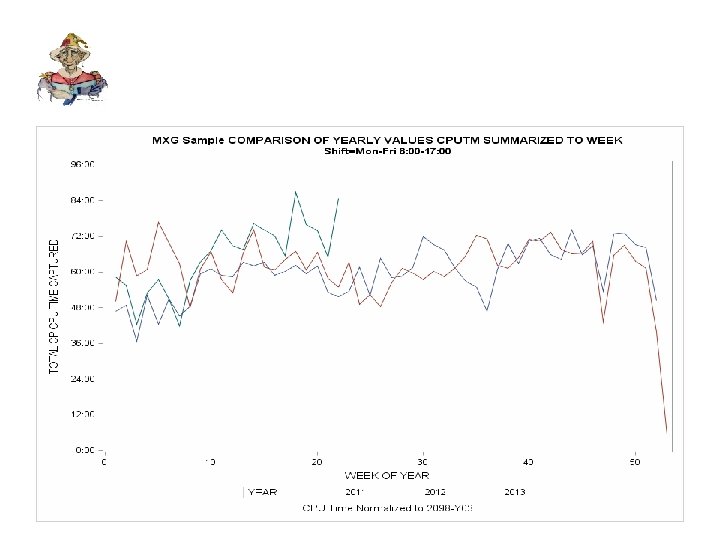
ANALCOMP filename html ‘/u/mvsdir/public_html’; ods graphics on/height=7 in width=9 in imagename='cpuyears' outputfmt=gif; ods html path=html body='trending. html'; %analcomp(indata=rmfintrv, compintv=week, xaxis=HOUR, datetime=startime, summary=yes, incode=if system='SYSG'; cputm=cputm*su_sec/28070. 1784; cputm cpuziptm time 8. ; label shift='Shift'; , footnote=CPU Time Normalized to 2098 -Y 03, vars=cputm cpuziptm, company=MXG Sample, compare=26 jun 13, nrperiods=3 ); run;

ANALCOMP

ANALCOMP

ANALCOMP proc format; value $shift 'P'='Mon-Fri 8: 00 -17: 00' 'N'='Mon-Fri 17: 00 -8: 00' 'W'='Weekend'; filename html ‘/u/mvsdir/public_html’; ods graphics on/height=7 in width=9 in imagename='cpuyears‘ outputfmt=gif; ods html path=html body='trending. html'; %analcomp(indata=rmfintrv, sortby=shift, compintv=year, xaxis=week, datetime=startime, incode=if system='SYSG'; cputm=cputm*su_sec/28070. 1784; format shift $shift. cputm cpuziptm time 8. ; label shift='Shift'; , footnote=CPU Time Normalized to 2098 -Y 03, vars=cputm cpuziptm, company=MXG Sample, compare=01 jan 11, nrperiods=3 );

ANALCOMP

VMXGPRNT • Utility to print any SAS dataset with labels modified to include the variable name and/or create a comma delimited output (CSV).

VMXGPRNT – Parameters • SP_DSET – dataset to be printed – defaults to _LAST_ • SP_NOBS – number of OBS to be printed – defaults to 20 • SP_REMV – remove * from labels in CSV file – defaults to NO

VMXGPRNT – Parameters • TMPPRNT – destination for a temporary dataset – on z. OS it will be constructed and dynalloc’ed as a temporary dataset but on ASCII will be placed in your SASUSER directory. Defaults to TMPPRNT. SAS • BYLST – list of BY variables – defaults to a null string

VMXGPRNT – Parameters • VARLST – list of variables to be printed. Default is a null string which will print all variables • NOEXIMSG – suppresses various warnings/notes – default is YES • SP_OPNS – PROC PRINT options default is SPLIT=‘*’
; • Print PDB. DB")
VMXGPRNT – Example 1 • %VMXGPRNT(SP_DSET=PDB. DB 2 ACCT, SP_NOBS=3); • Print PDB. DB 2 ACCT

VMXGPRNT – Example 1

VMXGPRNT – Example 2 • Create a CSV file – – – • Filename csv ‘h: mxgvmxgprnt. csv’; ods csvall file=csv; %vmxgprnt(SP_DSET=PDB. DB 2 ACCT, SP_NOBS=3, sp_remv=Y); run; ods csvall close; run;

VMXGPRNT – Example 2

VMXGFIND • Utility that will find every OBS in every dataset where some condition is satisfied and make a copy/print the observations. • For example: – Find all obs where JOB=: ’CICS’

VMXGFIND – Parameters • PDB= LIBNAME to be searched – default is PDB – can be 1 or many • PDBOUT= where to put the output datasets – datasets here will be named DDNAME_dataset where DDNAME is the libname where they were found

VMXGFIND – Parameters • KEEPIN= a list of variables that are used in the comparison • FIND= the comparison – for example… – Job=: ’CICS’ – KEEPIN=STARTIME STRTTIME INTBTIME, – FIND= IF ('31 JAN 2010: 11: 12'DT LE STARTIME LE '31 JAN 2010: 22: 23: 24'DT ) OR ('31 JAN 2010: 11: 12'DT LE STRTTIME LE '31 JAN 2010: 22: 23: 24'DT ) – OR ('31 JAN 2010: 11: 12'DT LE INTBTIME LE '31 JAN 2010: 22: 23: 24'DT ) ; ,

VMXGFIND – Parameters • PRINT= default is NO – YES – print all the observations – NO – no print – xxx – print xxx observations

VMXGFIND • If PRINT=YES or xxx then VMXGPRNT is used to do the printing • Example 1: – %VMXGFIND(FIND=QWHSSSID=DBTB, PRINT=3);

VMXGFIND

VMXGSRCH • Utility that will find every observation in every dataset in every allocated SAS data library where the value of the observation contains some string. – Note: libraries must have been allocated either explicitly (LIBNAME statement) or by a DATA/PROC step.

VMXGSRCH – Parameters • LIBNAME= the libname to be searched. Default is a NULL string. _ALL_ will search allocated SAS data libraries (they don’t have to be MXG) and anything else will search that specific LIBNAME. Only LIBNAMEs that have been opened will be found!!!!! You may need to insert a LIBNAME on z. OS.

VMXGSRCH - Parameters • COPYTO= copy the datasets and observations that match to this LIBNAME • NOBS= the number of OBS to print – default is MAX • LOG= a large number of lines may be generated – LOG=NO suppresses them. Default is YES

VMXGSRCH - Parameters • VALUE – the value to search for • Results= what you want us to do PRINT – just print the obs/datasets that match COPYONLY – copy the datasets but don’t print COUNT – just produce a count of datasets/obs/variables that match LABEL – produce a list of variables/datasets where the value is in the label – FORMAT – produce a list of variables/datasets where the value is in the format – –
;")
VMXGSRCH – Example 1 • %VMXGSRCH( LOG=NO, RESULTS=COUNT, VALUE=D 2 DD, LIBNAME=PDB);

VMXGSRCH- Example 1
;")
VMXGSRCH – Example 2 • %VMXGSRCH( LOG=NO, RESULTS=PRINT, NOBS=2, VALUE=D 2 DD, LIBNAME=PDB);

VMXGSRCH – Example 2
;")
VMXGSRCH – Example 3 • %VMXGSRCH( LOG=NO, RESULTS=PRINT, NOBS=2, VALUE=D 2 DD, LIBNAME=PDB, COPYTO=WORK);

VMXGSRCH – Example 3
;")
VMXGSRCH – Example 4 • %VMXGSRCH( LOG=NO, RESULTS=COPYONLY, VALUE=D 2 DD, LIBNAME=PDB, COPYTO=WORK);

VMXGSRCH – Example 4
; • NOTE: Values are case sensitive")
VMXGSRCH – Example 5 • %VMXGSRCH(VALUE=CPU, RESULTS=LABEL); • NOTE: Values are case sensitive

VMXGSRCH – Example 5
;")
VMXGSRCH – Example 6 • VMXGSRCH(VALUE=TIME, RESULTS=FORMAT);

VMXGSRCH – Example 6

READDB 2 • MXG supplied macro that generates the code to read all of the different types of DB 2 SMF data (all IFCIDs). It has been ‘enhanced’ to make a copy of the SMF data and allow for selection based on reading the record headers only which makes it very fast.

READDB 2 • For a full list of parameters and usage see READDB 2 member in the MXG SOURCLIB • Concentration here will be on selection parameters and copying of SMF data

READDB 2 • SMFOUT= DDNAME to which SMF data will be copied – if blank no copy is made • COPYONLY= YES/NO – only copy SMF data do not format SAS datasets – Useful to make mini-SMF files to feed to DB 2 PM or send off to vendors • PDBOUT= DDNAME to which SAS datasets are written (WORK is default if left blank)

READDB 2 - Parameters • • SYSTEM – list of systems PLAN – list of plan names AUTHID – list of authorization IDs CORRID – list of correlation IDs CONNID – list of connection IDs DB 2 – list of DB 2 subsystems CONNTYPE – list of connect types

READDB 2 - Parameters • TRANNAME – list of end-user transaction names • PACKAGE – list of package names • SMFBEGIN =SAS datetime constant – starting point of data • SMFEND – SAS datetime constant – end point of data – SAS datetime constants are of the form 01 sep 10: 01: 30: 00 – no quotes are needed

READDB 2 • All values in lists separated by spaces • All parameters separated by commas (except the last one) • All values are automatically wild carded – that is, however many bytes are in the value is the length of the compare • SMFBEGN= earliest time in form ddmmmyy: hh: mm: ss or 10 OCT 08: 15: 00 • SMFEND= latest time in same form
; – Copy records where TRANNAME starts with")
READDB 2 • %READDB 2(TRANNAME=OLB_DISP, COPYONLY=YES, SMFOUT=SMFOUT); – Copy records where TRANNAME starts with OLB_DISP to SMFOUT DD but do not create SAS datasets • %READDB 2(TRANNAME=OLB, PDB=WORK, SMFOUT=SMFOUT); – Copy records where TRANNAME starts with OLB and also place them in SAS datasets in the WORK dataset

VMXGSUM • Generalized summarization of ANY SAS dataset – – – – Uses PROC MEANS to do summarization SORTs data Allows for changes in input and output data Optimizes variables kept Carries labels and formats thru summarization Allows for long variable names Allows for normalization of variables and changing time intervals

VMXGSUM • Common in reporting: – DATA xxxx; – SET yyyy; – PROC SORT DATA=xxxx; – PROC MEANS DATA=XXXX OUT=zzzz; – DATA final; – SET zzzz;

VMXGSUM • VMXGSUM is a short-hand way of coding a repetitive set of commands. • Used extensively internally in many MXG members but especially common in ASUM**** and TRND**** members.
 name – OUTDATA= output dataset")
VMXGSUM - SYNTAX • %VMXGSUM( – INDATA= input dataset(s) name – OUTDATA= output dataset name – SUMBY= list of variables by which data should be sorted – INCODE= a stub of SAS code executed during the first data step – OUTCODE= a stub of SAS code executed during the final data step

VMXGSUM - SYNTAX – INTERVAL= how to change the time interval. Valid values are: • QTRHOUR HALFHOUR THREEHR • MINUTE WEEK MONTH MYTIME – DATETIME= the variable name of the variable containing the datetime value on which INTERVAL= will be applied – SYNC 59= if your time is synched to 59 minutes, will add 60 seconds before calculating interval if set to YES

VMXGSUM - SYNTAX • ID= list of variables that will be carried forward as ID values • AUTONAME=YES/NO AUTONAME = YES says to use the autonaming functions of SAS V 8 to name the output variables. – This allows the specification of the same variable name in multiple lists but changes the output variable name to variable_suffix where suffix is the name of the function performed on the variable.

VMXGSUM - SYNTAX • • SUM= list of variables to be summed MAX= list of variables to be maxxed MIN= list of variables to be minned MEAN= list of variables to be meaned P 1= list of variables to get percentile 1 P 5= 5 th percentile variables P 10= 10 th percentile variables

VMXGSUM - SYNTAX – P 25 P 50 P 75 P 90 P 95 P 99 - percentile values – STD - Standard Deviation – VAR - variance – CV - coefficient of variance – STDERR - Standard error – KURTOSIS - Kurtosis – T - T value

VMXGSUM - Syntax • NORM 1 -NORM 99 - normalization of data. Maintaining rates as rates and not averages of averages. On the front-end, the rate has to be multiplied by the duration and on the back end divided again to recalculate the correct rate.

VMXGSUM - SYNTAX – NORM 1 -NORM 99 - syntax • rate 1 rate 2 rate 3…ratex/duration • List the variables to be normalized followed by a / then the variable to be used to do the normalization.

VMXGSUM - SYNTAX • There are other parameters. See the documentation in the member for usage and the member ADOCSUM.

VMXGSUM - Example 1 • Summarize the dataset TYPETMNT by DEVICE and TMNTTIME calculating average mount delay and the total number of mounts per quarter hour. %vmxgsum( indata=pdb. typetmnt, outdata=tapemnts, sumby=device tmnttime, interval=qtrhour, datetime=tmnttime, mean=tapmnttm, freq=mounts );

VMXGSUM - Example 2 • Summarize the Goal Mode type 72 records for the TSO service class calculating the average response time, the number of transactions at one hour intervals by period.

VMXGSUM - Example 2 %VMXGSUM( INDATA=PDB. TYPE 72 GO, OUTDATA=TSOSUM, SUMBY=STARTIME PERIOD, INCODE= IF SRVCLASS=‘TSO’; , SUM=RESPAVG NUMTRAN, NORM 1=RESPAVG/NUMTRAN, INTERVAL=HOUR, DATETIME=STARTIME );

VMXGSUM Usage Notes • NORMx operands must be contiguous starting at 1. That is, you cannot have NORM 1 and NORM 3 without a NORM 2.

VMXGSUM Usage Notes • The first data step is almost always converted to a VIEW rather than a real data step. • KEEPALL=NO is resource intensive and not really needed except in odd cases. KEEPALL=YES is much preferred. The keep lists on all output datasets are optimized regardless of KEEPALL setting.

Why VMXGSUM? • So why not just use PROC MEANS with CLASS operands? • VMXGSUM in tests is usually much more efficient and in some cases will do the summarization where using PROC MEANS or PROC SUMMARY with CLASS operands runs out of memory. • This is especially true with the current release of SAS (9. 1. 3 SP 4) on z. OS which is defaulting to using THREADS.

ANALCNCR • Counts concurrent events. How many of something were happening at the same time.

ANALCNCR - History • Method used in original release of MXG: – DO TIME=BEGIN TO END BY 5; – OUTPUT; – END; – Then add up all the observations with a given value of TIME. Created a HUGE number of observations and was cumbersome.

ANALCNCR - History • Method used with ANALCNCR: – TIME=BEGIN; COUNT=1; OUTPUT; – TIME=END; COUNT=-1; OUTPUT; – Now add up the counts by time and you are done (basically. ) Many many fewer observations.

ANALCNCR - History • If there are three tape allocations: – Allocation 1 begins at 08: 00 ends at 08: 30 – Allocation 2 begins at 08: 15 ends at 08: 25 – Allocation 3 begins at 08: 20 ends at 08: 45

ANALCNCR - History • MAX of 3 concurrent allocations – – – 15 minutes of 1 5 minutes of 2 5 minutes of 3 5 minutes of 2 15 minutes of 1 • Old method – – Allocation 1 - 1800/5=360 obs Allocation 2 - 600/5=120 obs Allocation 3 - 1500/5=300 obs Total = 780 obs • New Method – – Each allocation is 2 OBS Total = 6

ANALCNCR - Example 1 • How many jobs are running concurrently in class A average and max. %ANALCNCR(INDATA=PDB. JOBS, OUTSUMRY=RUNTIME, SUMBY=JOBCLASS, INCODE=IF TYPETASK=‘JOB’; , INTERVAL=QTRHOUR, STARTIME=JINITIME, ENDTIME=JTRMTIME, OTCODESM= AVGRUN=CONCURNT/DURATM; RENAME MAXCNCR=MAXRUN; ); PROC PRINT; ID JOBCLASS TIMESTMP; VAR AVGRUN MAXRUN;

ANALCNCR - Example 2 • Now suppose you want the INPUT QUEUE time for the same job class. %ANALCNCR(INDATA=PDB. JOBS, OUTSUMRY=QUETIME, SUMBY=JOBCLASS, INCODE=IF TYPETASK=: ’JOB’; , INTERVAL=QTRHOUR, STARTIME=READTIME, ENDTIME=JINITIME, OTCODESM= AVGQUE=CONCURNT/DURATM; RENAME MAXQUE=MAXRUN; ); PROC PRINT; ID JOBCLASS TIMESTMP; VAR AVGQUE MAXQUE;

ANALCNCR - Example 3 • Now put the two outputs together DATA JOBSTAT; MERGE RUNTIME QUETIME; BY JOBCLASS TIMESTMP; PROC PRINT; ID JOBCLASS TIMESTMP; VAR AVGQUE AVGRUN MAXQUE MAXRUN;

ANALCAPD Can you save money by capping the MSU’s consumed? Billing is based on the peak of the rolling 4 hour MSU average Rolling average will (almost) always lag behind actual usage So, you can set a cap lower than the actual peak and possibly reduce software billing • ANALCAPD will let you ‘play’ with values to find a happy MSU value that allows work to run while reducing the peak MSU value • •

ANALCAPD • Uses the ASUMCEC dataset in the PDB as input • Best granularity is when you match CECINTRV to INTERVAL in ASUM 70 PR

ANALCAPD – Parameters • PDB=PDB – where is the ASUMCEC data • GRAPHICS=YES – use SAS/GRAPH (it will detect if it is not there) • DEFCAP= the MSU value you want to ‘model’ • CECINTRV=HOUR – the CECINTRV value in use – QTRHOUR HALFHOUR etc

ANALCAPD - Results

ANALCAPD – Results • Black line is current capacity • Cyan line is current cap (in this case there is not one) • Blue line is actual usage • Green line is rolling 4 hour average • Red * are the intervals where the CEC would have been capped

- Slides: 178