Mutation Origin of genetic variation sources of new

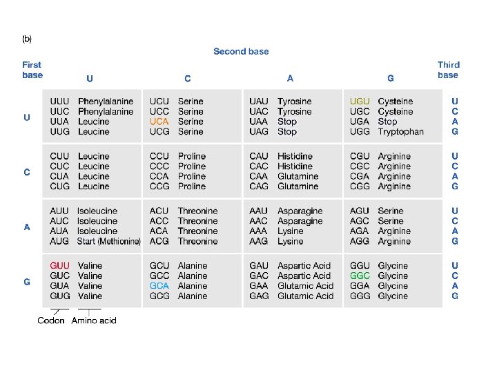
Mutation: Origin of genetic variation sources of new alleles rate and nature of mutations sources of new genes highly repeated functional sequences

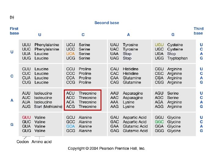
new alleles arise from changes in DNA sequence point mutations deletions frameshift mutations insertions transposition inversion or translocation breakpoints point mutations may either be synonymous substitutions -- no change in amino acid identity replacement substitutions -- changed amino acid

60 -70% of mutations are transitions (vs. exp. 33%)

Transition Resistant

Basic

Polar Acidic

mutation rates vary considerably among species

mutation rates vary considerably among genes within a species

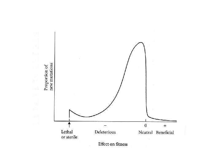
most mutations are deleterious -- C. elegans (Vassilieva et al. 2000)

most mutations are deleterious WHY? ? If all mechanisms were nearly ‘perfect’ any change would be detrimental. Maybe Best place 50% chance of improvement

most mutations are deleterious WHY? ? If all mechanisms were nearly ‘perfect’ any change would be detrimental. Maybe Suppose two dimensions Chance of improvement Less than 50% With many more dimensions the chance of improvement goes to zero.

most mutations are only slightly deleterious

Origins of new genes duplications pseudogenes Repeated arrays Function lost Mutations accumulate novel functions e. g. Tandem repeats of r. RNA genes Absence of variation in repeats Suggests functional requirements Expression patterns Exon shuffling Internal repeats

New genes via internal duplications: antifreeze glycoprotein in Antarctic Toothfish (Dissostichus mawsoni) waters of the Antarctic Ocean -1. 9 o. C most fish freeze at -1. 0 o. C to – 0. 7 o. C

ancestral trypsinogen gene antifreeze glycoprotein gene (from Graur & Li 2000)

New genes via exon shuffling: tissue plasminogen activator evolves from four unrelated genes protease kringle (plasminogen) epidermal growth factor fibronectin type-1 (from Graur & Li 2000)

new alleles are produced by mutation most mutations are slightly deleterious duplication is the most important mechanism for producing new genes

Populations are affected by two sets of processes: 1. Genetic -- mutation, recombination, independent assortment, transposition, meiotic drive 2. Ecological -- changes in population size, dispersal, mating system, environmental variation How do these processes affect population genetic variation ?

plumage variation in the snow goose, Chen caerulescens white phase blue phase

morphological variation in Panaxia dominula P. d. dominula c dc d P. d. medionigra c dc b P. d. bimacula c bc b

protein electrophoresis

PO 7 275 kb Microsatellite loci for Pogonomyrmex occidentalis PO 8 250 kb PO 3 160 kb PO 1 175 kb

Quantifying population genetic variation: # particular genotype frequency = total number of individuals allele frequency = # particular allele total number of alleles by the law of proportions, both genotype and allele frequencies always sum to one

genotype A 1 A 1 A 1 A 2 A 2 A 2 number 670 200 130 genotype frequency 670 1000 200 1000 130 1000 geno freq. 0. 67 0. 20 0. 13 frequency of A 1 = 0. 67 + 1 2 (0. 20) = 0. 77 frequency of A 2 = 0. 13 + 1 2 (0. 20) = 0. 23

genotype A 1 A 1 A 1 A 2 A 2 A 2 number 670 200 130 Genotype frequency 0. 67 0. 20 0. 13 Allele frequencies: A 1 = 0. 77 A 2 = 0. 23 What are the expected genotype frequencies? A 1 A 1 A 1 A 2 A 2 A 2 . 77 x. 77 2 x(. 77 x. 23) . 23 x. 23 . 59 . 35 . 05

genotype A 1 A 1 Genotype frequency G 1 Allele frequency A 1 A 2 A 2 A 2 G 3 p A 2 q Expected genotype frequencies: p 2 Remember: 2 pq q 2 p+q = 1 Therefore (p+q) 2 = 12 , or p 2 + 2 pq + q 2 =1

When the observed genotype frequencies equal the expected genotype frequencies the population is said to be in Hardy-Weinberg Equilibrium

Hardy-Weinberg Equilibrium In the presence of certain conditions, the genotype frequencies of a population will be stable over time, and will be directly predictable from the allele frequencies. If the population is not at equilibrium, it will achieve it after one generation of random mating. Assumes: no mutation, no selection, infinite population size, no gene flow, random mating Null model for describing population genetic variation

How do we know whether a population is in HWE: genotype MM MN NN number 60 20 20 obs. gen. fr. 0. 6 0. 2 f (M) = 0. 6 + 0. 1 = 0. 7 f (N) = 0. 2 + 0. 1 = 0. 3 exp. gen. fr. f (M)2 2 f (M)f (N)2 (0. 7)2 0. 49 49 2(0. 7)(0. 3)2 0. 42 0. 09 42 9 DO NOT say: (0. 7)2 + 2(0. 7)(0. 3) + (0. 3)2 = 1, therefore HWE.

Compare observed and expected genotype distributions with a goodness of fit chi-square test with n-1 degrees of freedom (n = number of categories) One additional degree of freedom is lost when estimating allele frequencies dof = (n - 2) c 2 dof = S (observed # - expected #)2 (expected #) for the data on the previous page: c 2 Look up in Table: critical values df 1 2 3 2 = 27. 4 0. 05 3. 84 6. 0 7. 82 . 025 5. 02 7. 38 9. 35 0. 01 6. 64 9. 21 11. 35 0. 005 7. 88 10. 6 12. 84

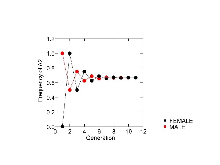
HWE and sex-linked genes autosomes: half of the alleles in each sex chromosomes: two-thirds of the alleles in the homogametic (XX) sex if males are homogametic, A 1 A 1 A 1 A 2 males A 2 A 2 A 1/ A 2/ females allele frequencies are sex-specific: pm, qm and pf, qf

Under random mating: qm ’ = qf ’ = 1 2 (qm + qf) males get an X-chromosome from each parent qm females get their only X-chromosome from their father qm’- qf’ = ½ qm + ½ qf - qm = - ½(qm- qf ) pm + 1 3 pf q = > > p = 2 3 qm + 13 qf

genetic diversity characterizes most natural populations Hardy-Weinberg Equilibrium represents a null model for the evolution of genotype frequencies basis for mathematically examining the effects of: mutation, selection, genetic drift, gene flow, and non-random mating dynamics of HWE differ for sex-linked genes