Muon Tomography Algorithms for Nuclear Threat Detection R

Muon Tomography Algorithms for Nuclear Threat Detection R. Hoch, D. Mitra, M. Hohlmann, K. Gnanvo

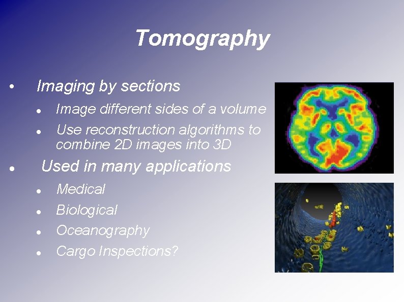
Tomography • Imaging by sections Image different sides of a volume Use reconstruction algorithms to combine 2 D images into 3 D Used in many applications Medical Biological Oceanography Cargo Inspections?

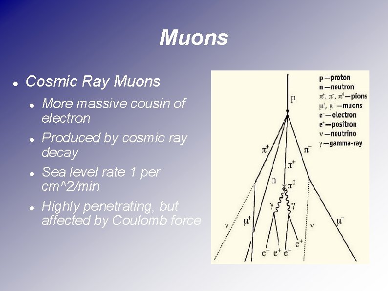
Muons Cosmic Ray Muons More massive cousin of electron Produced by cosmic ray decay Sea level rate 1 per cm^2/min Highly penetrating, but affected by Coulomb force

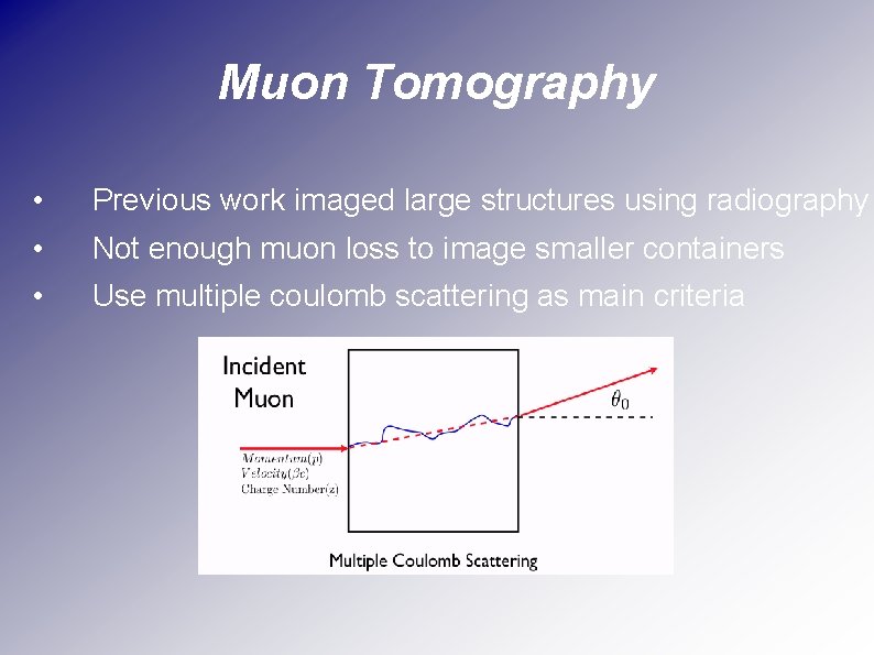
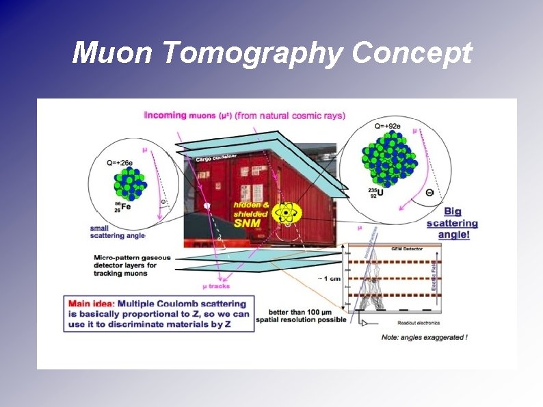
Muon Tomography • Previous work imaged large structures using radiography • Not enough muon loss to image smaller containers • Use multiple coulomb scattering as main criteria

Muon Tomography Concept

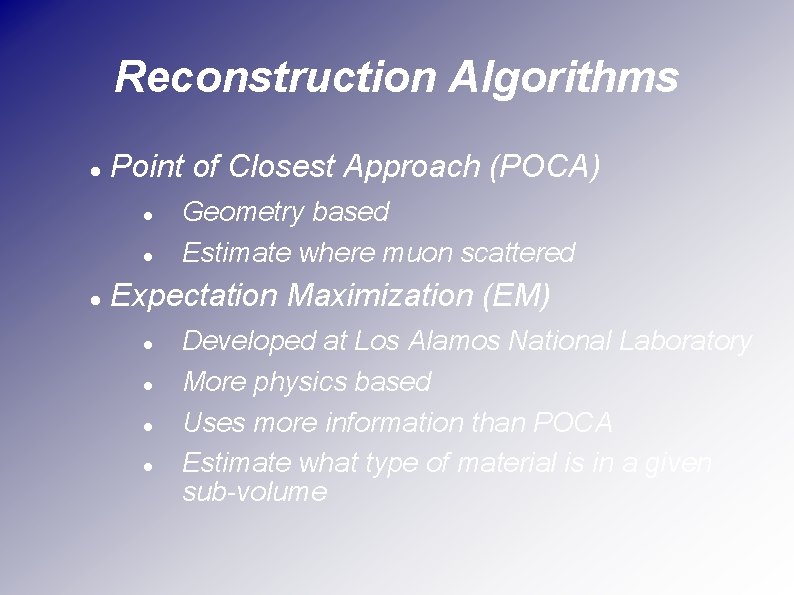
Reconstruction Algorithms Point of Closest Approach (POCA) Geometry based Estimate where muon scattered Expectation Maximization (EM) Developed at Los Alamos National Laboratory More physics based Uses more information than POCA Estimate what type of material is in a given sub-volume

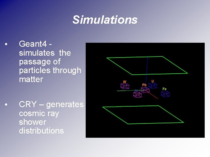
Simulations • Geant 4 simulates the passage of particles through matter • CRY – generates cosmic ray shower distributions

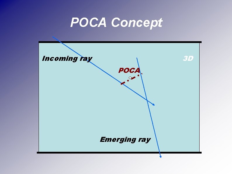
POCA Concept Incoming ray 3 D POCA Emerging ray

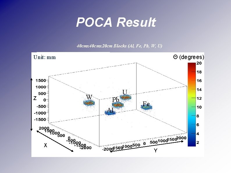
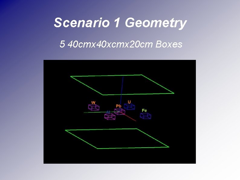
POCA Result 40 cmx 20 cm Blocks (Al, Fe, Pb, W, U) Θ (degrees) Unit: mm W Z X Pb Al U Fe Y

POCA Discussion Pro’s Fast and efficient Can be updated continuously Accurate for simple scenario’s Con’s Doesn’t use all available information Unscattered tracks are useless Performance decreases for complex scenarios

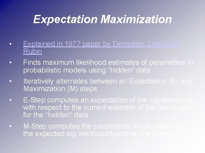
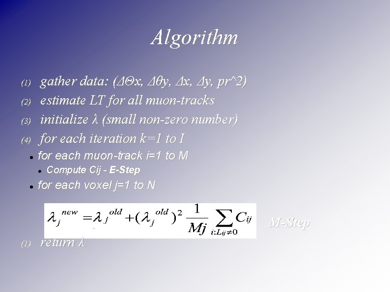
Expectation Maximization • Explained in 1977 paper by Dempster, Laird and Rubin • Finds maximum likelihood estimates of parameters in probabilistic models using “hidden” data • Iteratively alternates between an Expectation (E) and Maximization (M) steps • E-Step computes an expectation of the log likelihood with respect to the current estimate of the distribution for the “hidden” data • M-Step computes the parameters which maximize the expected log likelihood found on the E step

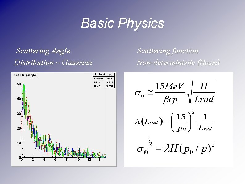
Basic Physics Scattering Angle Distribution ~ Gaussian Scattering function Non-deterministic (Rossi)

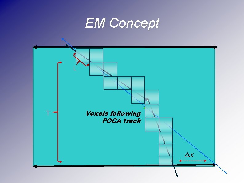
EM Concept L T Voxels following POCA track

Algorithm (1) (2) (3) (4) gather data: (ΔΘx, Δθy, Δx, Δy, pr^2) estimate LT for all muon-tracks initialize λ (small non-zero number) for each iteration k=1 to I for each muon-track i=1 to M Compute Cij - E-Step for each voxel j=1 to N M-Step (1) return λ

Scenario 1 Geometry 5 40 cmx 40 xcmx 20 cm Boxes

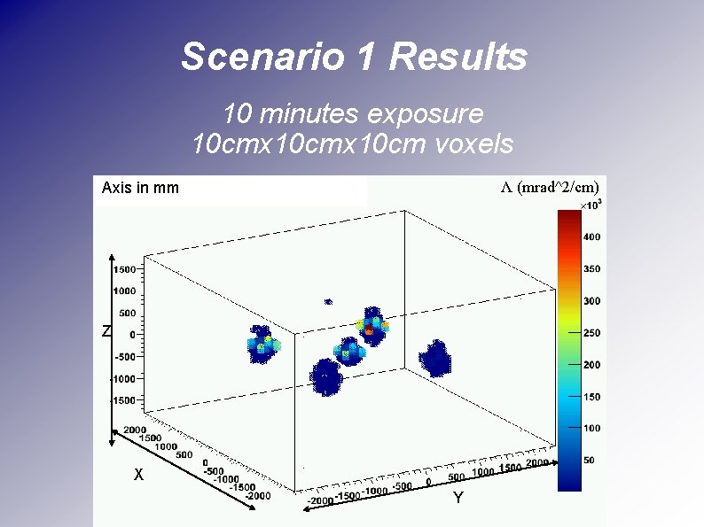
Scenario 1 Results 10 minutes exposure 10 cmx 10 cm voxels Axis in mm Λ (mrad^2/cm) Z X Y

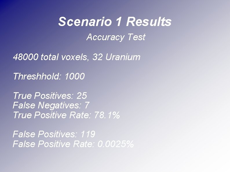
Scenario 1 Results Accuracy Test 48000 total voxels, 32 Uranium Threshhold: 1000 True Positives: 25 False Negatives: 7 True Positive Rate: 78. 1% False Positives: 119 False Positive Rate: 0. 0025%

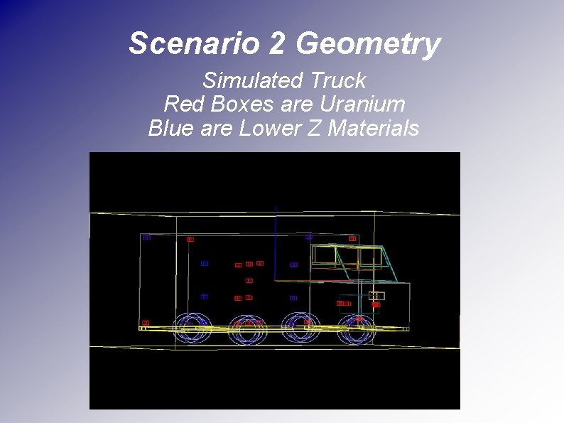
Scenario 2 Geometry Simulated Truck Red Boxes are Uranium Blue are Lower Z Materials

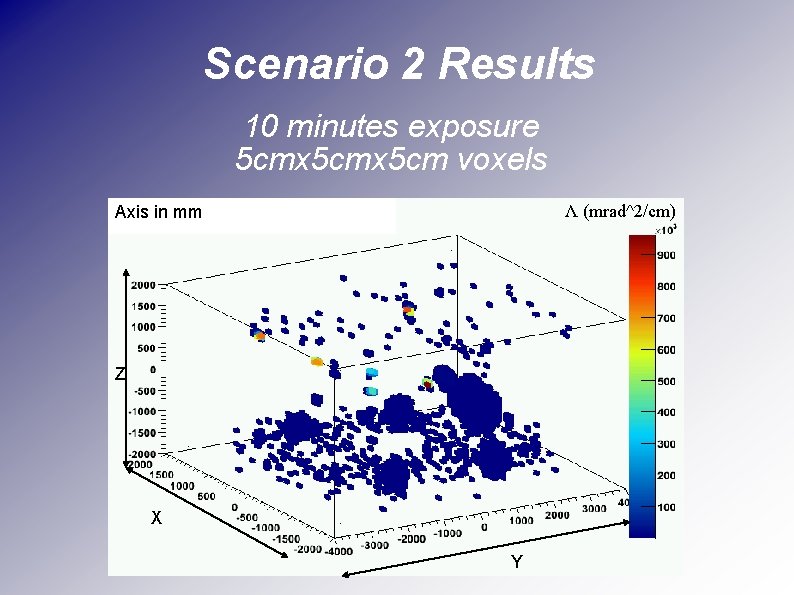
Scenario 2 Results 10 minutes exposure 5 cmx 5 cm voxels Axis in mm Λ (mrad^2/cm) Z X Y

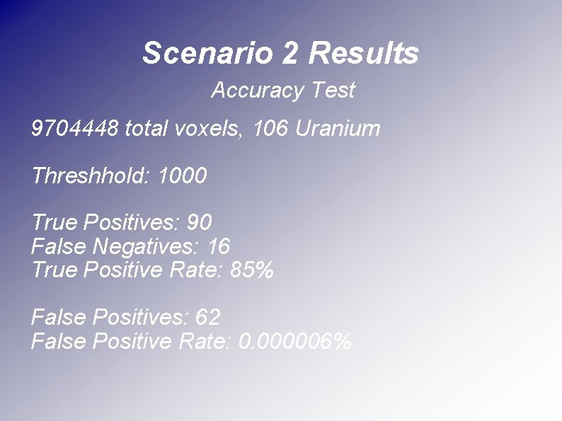
Scenario 2 Results Accuracy Test 9704448 total voxels, 106 Uranium Threshhold: 1000 True Positives: 90 False Negatives: 16 True Positive Rate: 85% False Positives: 62 False Positive Rate: 0. 000006%

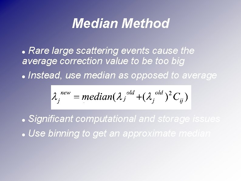
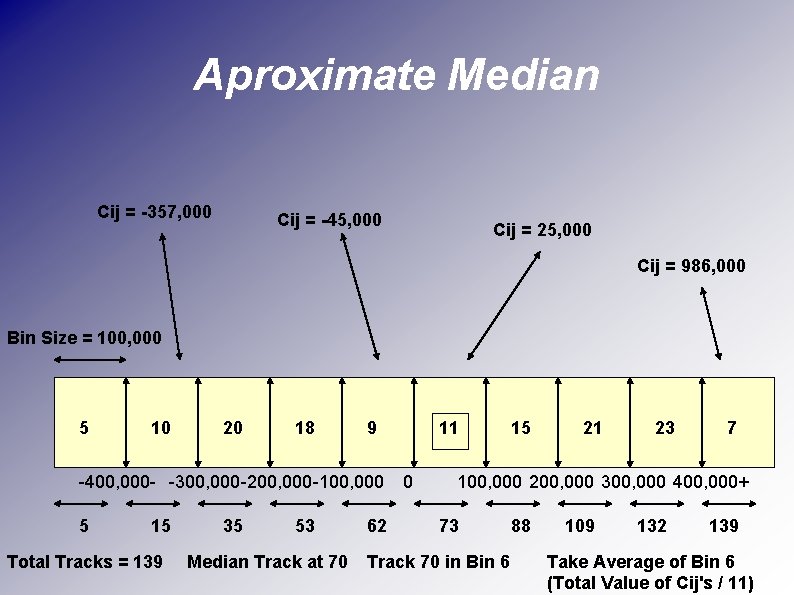
Median Method Rare large scattering events cause the average correction value to be too big Instead, use median as opposed to average Significant computational and storage issues Use binning to get an approximate median

Aproximate Median Cij = -357, 000 Cij = -45, 000 Cij = 25, 000 Cij = 986, 000 Bin Size = 100, 000 5 10 20 18 9 -400, 000 - -300, 000 -200, 000 -100, 000 5 15 Total Tracks = 139 35 53 Median Track at 70 62 11 0 15 21 23 7 100, 000 200, 000 300, 000 400, 000+ 73 Track 70 in Bin 6 88 109 132 139 Take Average of Bin 6 (Total Value of Cij's / 11)

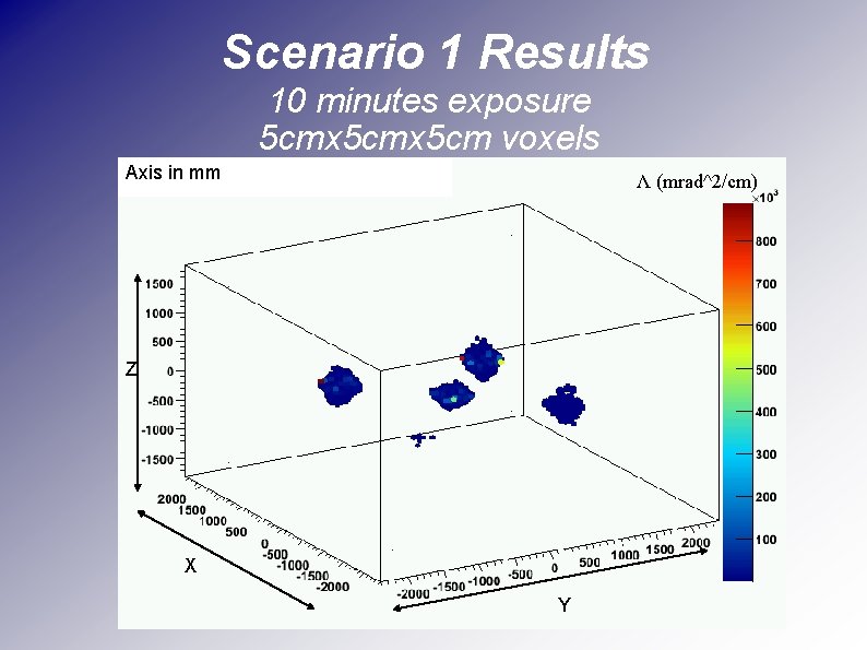
Scenario 1 Results 10 minutes exposure 5 cmx 5 cm voxels Axis in mm Λ (mrad^2/cm) Z X Y

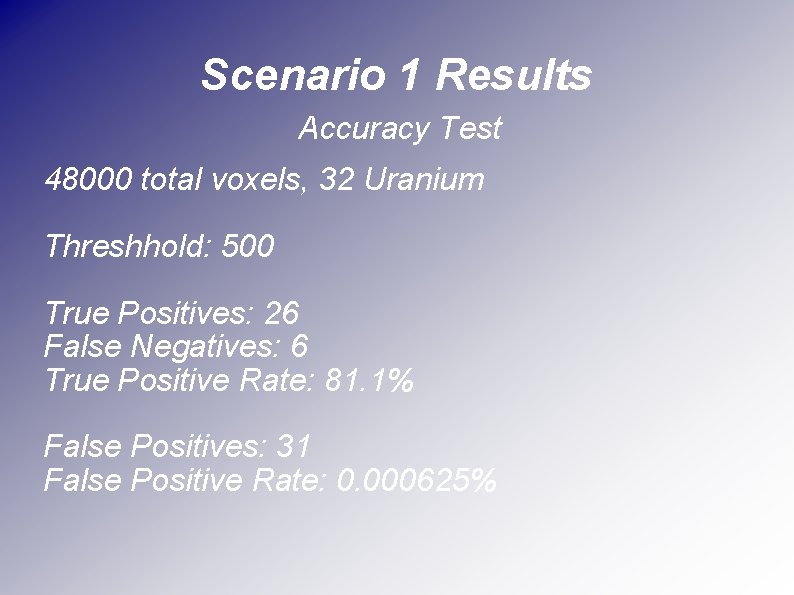
Scenario 1 Results Accuracy Test 48000 total voxels, 32 Uranium Threshhold: 500 True Positives: 26 False Negatives: 6 True Positive Rate: 81. 1% False Positives: 31 False Positive Rate: 0. 000625%

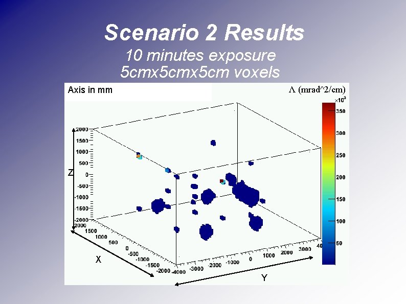
Scenario 2 Results 10 minutes exposure 5 cmx 5 cm voxels Axis in mm Λ (mrad^2/cm) Z X Y

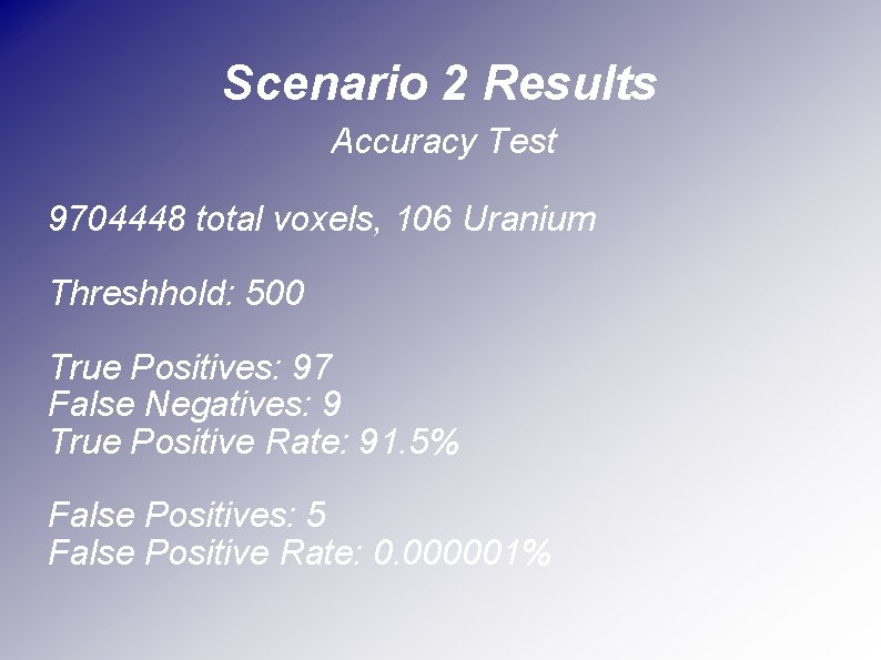
Scenario 2 Results Accuracy Test 9704448 total voxels, 106 Uranium Threshhold: 500 True Positives: 97 False Negatives: 9 True Positive Rate: 91. 5% False Positives: 5 False Positive Rate: 0. 000001%

Future Work Improvement of absolute lambda values Real-time EM Analysis of complex scenarios

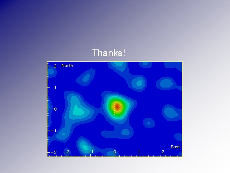
Thanks!

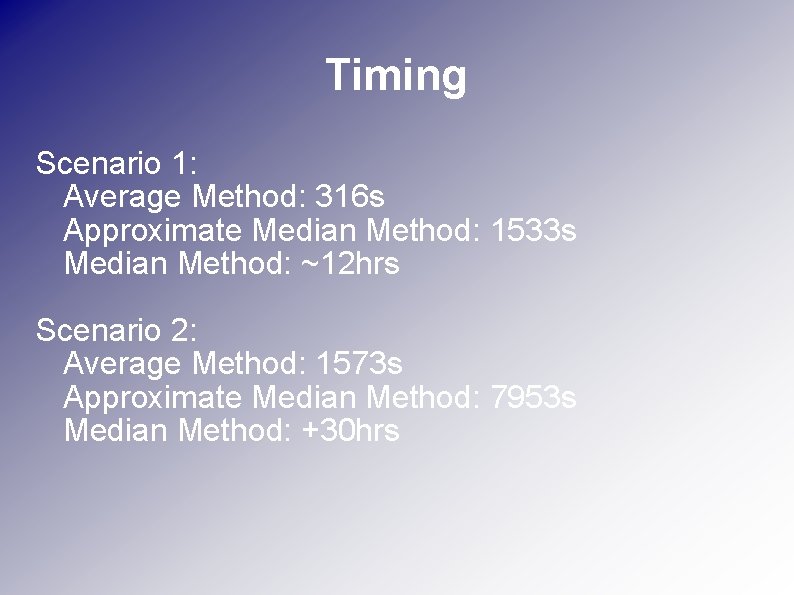
Timing Scenario 1: Average Method: 316 s Approximate Median Method: 1533 s Median Method: ~12 hrs Scenario 2: Average Method: 1573 s Approximate Median Method: 7953 s Median Method: +30 hrs

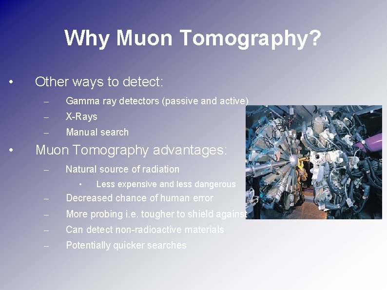
Why Muon Tomography? • • Other ways to detect: – Gamma ray detectors (passive and active) – X-Rays – Manual search Muon Tomography advantages: – Natural source of radiation • Less expensive and less dangerous – Decreased chance of human error – More probing i. e. tougher to shield against – Can detect non-radioactive materials – Potentially quicker searches