MUO Introduction Based on mechanical force To mix
 • Based on mechanical force: • • To mix different components To")
MUO (Introduction) • Based on mechanical force: • • To mix different components To separate a specified component from a mixture Size reduction and enlargement Enhance mass and heat transfer (drying, absorption, etc. ) • Most frequent mechanical unit operations (MUO): • Size reduction, screening, sedimentation, fluidization, filtration, centrifugation, cyclones, magnetic separation, electro-static precipitators, floatation, solid transportation , mixing Solomon Bogale Chemical Eng'g Department
 • If not all, most unit operations depend on particle size")
MUO (Intro…particle size) • If not all, most unit operations depend on particle size range of the material involved. • Particles resulting from size reduction (naturally): – Are not perfectly spherical – Contain (more or less) broad range of particle sizes • Two basic challenges – How to characterize a particle of arbitrary shape by one single particle size? – How to describe a particle size distribution? Solomon Bogale Chemical Eng'g Department
 • Particle size measuring methods – Microscopic techniques are based")
MUO (Particle size measurement) • Particle size measuring methods – Microscopic techniques are based on direct observation (used as a reference method) – Light microscopy (>0. 5 m) – (Scanning) electron microscopy (>5 nm) – Sieving – Dry sieving (50 m – 10 cm) – Wet sieving (>20 m) • Performed in a range of standard sieves Solomon Bogale Chemical Eng'g Department ysis anal e g a Im que techni
 • Aperture size is the dimension of the opening •")
MUO (Particle size measurement) • Aperture size is the dimension of the opening • Mesh number is the number of openings per inch e. g. 200 mesh = 200 openings/inch = 74 m/opening The results of the sieve analysis can be represented by • histogram • differential distribution • cumulative distribution • The particle size of the material remaining between the two sieves is mostly accepted to be halve of the sum of the two sieve openings Solomon Bogale Chemical Eng'g Department

Sieve standards: Mesh size vs. aperture size
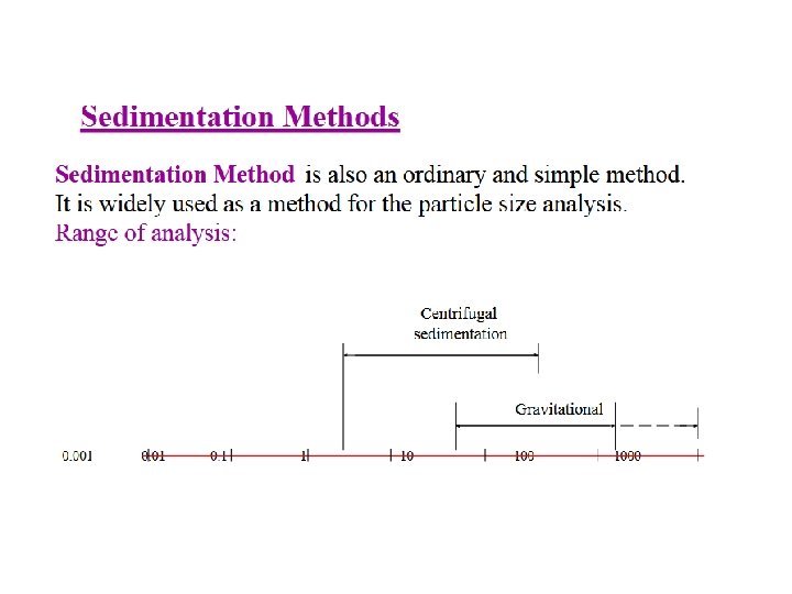
 • Sedimentation – Sedimentation in a gravitational field (50 m")
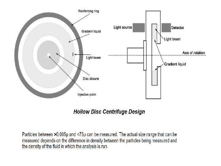
MUO (Particle size measurement) • Sedimentation – Sedimentation in a gravitational field (50 m – 0. 5 m ) – Detection techniques • • • Photo X-ray Gravimetric Densitometric Pipette-sedimentometry – Sedimentation in a centrifugal field is applicable (1 m – 1 nm) Solomon Bogale Chemical Eng'g Department
 • Electrical sensing zone (coulter counter) – Suspension passed through")
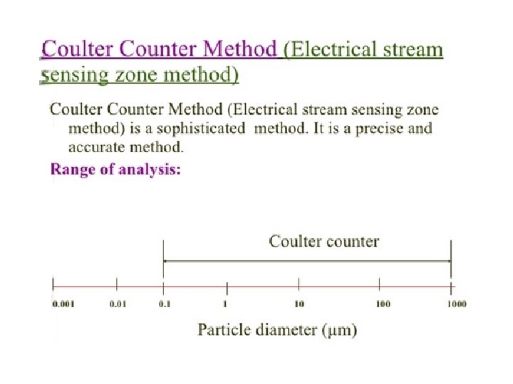
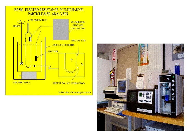
MUO (Particle size measurement) • Electrical sensing zone (coulter counter) – Suspension passed through capillary conductivity cell – Size range (1000 m – 0. 1 m) • Light scattering techniques – Classical light scattering according to Rayleigh or Mietheory – Laser-Fraunhofer-diffraction (1 m -1800 m) – Laser-photon correlation spectroscopy(3 nm-3 m) Solomon Bogale Chemical Eng'g Department
 Electrical sensing zone (coulter counter) • Helps to count the particles")
MUO(Particle size measurement) Electrical sensing zone (coulter counter) • Helps to count the particles • Based on the resistance b/n the electrodes
 Light scattering techniques Solomon Bogale Chemical Eng'g Department")
MUO(Particle size measurement) Light scattering techniques Solomon Bogale Chemical Eng'g Department
 Light scattering techniques")
MUO(Particle size measurement) Light scattering techniques
 Light scattering techniques")
MUO(Particle size measurement) Light scattering techniques
 • Particle size characterization: – Spherical particles have one single")
MUO (Particle size characterization) • Particle size characterization: – Spherical particles have one single dimension (i. e. the diameter ) – Particles of arbitrary shape are assigned a diameter of an equivalent sphere. The equivalency can be based on: • Surface area of the particle (a 1) Area e qu sphere ivalent diamet er Solomon Bogale Chemical Eng'g Department
 • Volume of the particle (V 1): ivalent u q")
MUO (Particle size characterization) • Volume of the particle (V 1): ivalent u q e e volum eter m a i d e r sphe • Specific surface per unit volume of the particle (S’): Solomon Bogale Chemical Eng'g Department
 • Sedimentation velocity of the particle (u): lent a v")
MUO (Particle size characterization) • Sedimentation velocity of the particle (u): lent a v i u q e stokes eter m a i d e r sphe • Sieve opening = mesh equivalent sphere diameter – The diameter of the various equivalent spheres is different. Hence, irregularly shaped particle doesn’t have an unequivocal size. Solomon Bogale Chemical Eng'g Department
 • Equivalent sphere diameters of a cube of edge L")
MUO (Particle size characterization) • Equivalent sphere diameters of a cube of edge L Equivalency Cube Sphere Surface Volume Vol. -spec. area Solomon Bogale Chemical Eng'g Department esd
 • Shape factors – Shape of the particles can be as")
MUO (Shape factors) • Shape factors – Shape of the particles can be as important as their size – Shape factor is derived from the ratio of two different equivalent sphere diameters: • Sphericity ( ) Solomon Bogale Chemical Eng'g Department
 • e. g. sphericity of a cube of edge L: •")
MUO (Shape factors) • e. g. sphericity of a cube of edge L: • Circularity ( ): Based on a projected area of the particle (found from image analysis) a 1 P and the perimeter of the projected area P. Solomon Bogale Chemical Eng'g Department
 • e. g. the circularity of a cube of edge L:")
MUO (Shape factors) • e. g. the circularity of a cube of edge L: Solomon Bogale Chemical Eng'g Department
 Solomon Bogale Chemical Eng'g Department")
MUO (size distribution analysis) Solomon Bogale Chemical Eng'g Department

At t = tf Total mass of the sample = 500 gm 0. 94 mm 0 gm 0. 84 mm 50 gm 0. 76 mm 50 gm 0. 68 mm 100 gm 0. 62 mm 100 gm 0. 56 mm 100 gm 0. 5 mm 60 gm 0. 4 mm 40 gm Pan 0 gm
 Dmi (gm) Dmi (%) Dfi (mm) Dmi/Dfi (mm)-1 Dmi (%)")
Sieve opening fi (mm) Dmi (gm) Dmi (%) Dfi (mm) Dmi/Dfi (mm)-1 Dmi (%) < 0. 4 0. 2 0 0 0. 4 < fi < 0. 5(0. 4+0. 5) =0. 45 40 (40/500)100 =8 (0. 5 -0. 4) =0. 1 (8/0. 1) =80 8+0 = 8 0. 5 < fi < 0. 56 0. 53 60 12 0. 06 200 12+8 = 20 0. 56 < fi < 0. 62 0. 59 100 20 0. 06 333 20+20 = 40 0. 62 < fi < 0. 68 0. 65 100 20 0. 06 333 20+40 = 60 0. 68 < fi < 0. 76 0. 72 100 20 0. 08 250 20+60 = 80 0. 76 < fi < 0. 84 0. 80 50 10 0. 08 125 10+80 = 90 0. 84 < fi < 0. 94 0. 89 50 10 0. 10 10+90 = 100 0 0 > 0. 94 Total = 500 0
 Dmi (gm) Dmi (%) Dfi (m) Dmi/Dfi (m)-1 Dmi (%)")
Sieve opening fi (m) Dmi (gm) Dmi (%) Dfi (m) Dmi/Dfi (m)-1 Dmi (%) < 0. 4 0. 2 e-3 0 0 0. 4 < fi < 0. 5(0. 4+0. 5)e-3 =4. 5 e-4 40 (40/500)100 =8 (0. 5 -0. 4)e-3 =1 e-4 (0. 08/1 e-4) =8 e 2 8+0 = 8 0. 5 < fi < 0. 56 5. 3 e-4 60 12 6 e-5 2 e 3 12+8 = 20 0. 56 < fi < 0. 62 5. 9 e-4 100 20 6 e-5 3. 33 e 3 20+20 = 40 0. 62 < fi < 0. 68 6. 5 e-4 100 20 6 e-5 3. 33 e 3 20+40 = 60 0. 68 < fi < 0. 76 7. 2 e-4 100 20 8 e-5 2. 5 e 3 20+60 = 80 0. 76 < fi < 0. 84 8 e-4 50 10 8 e-5 1. 25 e 3 10+80 = 90 0. 84 < fi < 0. 94 8. 9 e-4 50 10 1 e-4 1 e 3 10+90 = 100 0 0 > 0. 94 Total = 500 0

1. 20 E+10 Dni/Dfi 8. 00 E+09 number weighted differential distribution mass weighted differential distribution 3500 3000 2500 6. 00 E+09 2000 1500 4. 00 E+09 1000 2. 00 E+09 500 0. 00 E+00 2. 00 E-04 0 4. 00 E-04 6. 00 E-04 fi (m) 8. 00 E-04 1. 00 E-03 Dmi/Dfi 1. 00 E+10 4000

mass weighted cumulative distribution 120. 00% 100. 00% Dmi 80. 00% 60. 00% 40. 00% 20. 00% 0. 00 E+00 2. 00 E-04 4. 00 E-04 6. 00 E-04 8. 00 E-04 fi = average size (m) 1. 00 E-03
 mass of particles < sieve opening(%) mass of particles > sieve")
sieve openings (mm) mass of particles < sieve opening(%) mass of particles > sieve opening(%) 0. 4 0 0 100 0. 5 8 8 92 0. 56 12 20 80 0. 62 20 40 60 0. 68 20 60 40 0. 76 20 80 20 0. 84 10 90 10 0. 94 10 100 0
 Oversize cumulative distribution (>sieve opening) 120 cumulative distribution Dmi")
Undersize cumulative distribution (<sieve opening) Oversize cumulative distribution (>sieve opening) 120 cumulative distribution Dmi (%) 100 80 60 40 20 0 0 0. 2 0. 4 0. 6 fi = sieve opening (mm) 0. 8 1

Histogram of weight of sample against particle size q. The heights of the bars depends on the size of the sample you use Histogram of weight percent of sample against particle size q. The histogram is normalized by plotting percent of total weight vs. size class interval. Then, no matter how large or small the class interval, the total area under the histogram bars is unity. But still the height of the bars varies with the fineness of division of the size scale.

Normalized histogram of weight percent of sample per unit size interval against particle size q. When the vertical axis is weight percent divided by size interval, then the overall course of the tops of the bars is the same regardless of the fineness of subdivision. q. As you progressively decrease the size class interval, the bars get thinner, but the overall shape and size of the histogram stays the same. This is best visualized in a vertical line graph, with data plotted as vertical lines from the midpoints of the class intervals.

If you performed the limiting process for a smoothly continuous variable, you would get a limiting continuous curve toward which the successively finer histograms would tend. This is called the frequency distribution curve or frequency distribution function Cumulative distribution function showing weight percent of sample against particle size
 • Particle size distributions Number of particles of a given")
MUO (size distribution analysis) • Particle size distributions Number of particles of a given size -- number weighted PSD The length of particles of a given size --length weighted PSD The area of particles of a given size -- area weighted PSD The volume of particles of a given size -- volume weighted PSD – The mass of particles of a given size -- mass weighted PSD – – d. N/dlogf and d. M/dlogf Distributions 250 200 Number 150 Mass 100 50 0 10. 0 f (nm) 100. 0 1000. 0 number distribution is dominated by smaller particles, mass distribution is dominated by larger particles
 • For discrete particle size distribution, the number weighted distribution")
MUO (size distribution analysis) • For discrete particle size distribution, the number weighted distribution is written as ni/ i. Solomon Bogale Chemical Eng'g Department
 • For continuous particle size distributions: Solomon Bogale Chemical Eng'g")
MUO (size distribution analysis) • For continuous particle size distributions: Solomon Bogale Chemical Eng'g Department
 • In general, represents particle size distribution • Arbitrary PSD")
MUO (size distribution analysis) • In general, represents particle size distribution • Arbitrary PSD can be transformed into a number distribution by: Solomon Bogale Chemical Eng'g Department
 • The factor Fq and the exponent q correspond to:")
MUO (size distribution analysis) • The factor Fq and the exponent q correspond to: Q n l a v m Fq 1 1 /6 ( /6) Solomon Bogale Chemical Eng'g Department q 0 1 2 3 3
 • The integral value of provide the total value of")
MUO (size distribution analysis) • The integral value of provide the total value of Solomon Bogale Chemical Eng'g Department from 0 to
 • k-th moment of a function around the reference value")
MUO (size distribution analysis) • k-th moment of a function around the reference value is given by: Solomon Bogale Chemical Eng'g Department
 • k-th moment of a function around the origin is")
MUO (size distribution analysis) • k-th moment of a function around the origin is given by: • The 0 -th moment around the origin is the total value Solomon Bogale Chemical Eng'g Department
 • The integral or total value of may be written")
MUO (size distribution analysis) • The integral or total value of may be written as a function of the number weighted distribution • Weighted average diameters of any function is defined as
 • Combining the previous formulations, the weighted average diameter of")
MUO (size distribution analysis) • Combining the previous formulations, the weighted average diameter of the PSD can be written as: • Accordingly, if then (known as mass weighted average diameter)
 • -Equivalent average diameter given by: is")
MUO (size distribution analysis) • -Equivalent average diameter given by: is
 • Variance and standard deviation is defined as the ratio")
MUO (size distribution analysis) • Variance and standard deviation is defined as the ratio of the 2 -nd moment relative to the mean value to the 0 -th moment around the origin:
 Dmi fi (m) <4. 00 E-04 0 2. 00 E-04 4.")
sieve opening (m) Dmi fi (m) <4. 00 E-04 0 2. 00 E-04 4. 00 E-04 ---5. 00 E-04 0. 08 4. 50 E-04 5. 00 E-04 ---5. 60 E-04 0. 12 5. 60 E-04 ---6. 20 E-04 Dmi/Dfi Dni/Dfi 0 0 0 1. 00 E-04 8. 00 E+02 6. 33 E+05 6. 33 E+09 5. 30 E-04 6. 00 E-05 2. 00 E+03 5. 81 E+05 9. 68 E+09 0. 2 5. 90 E-04 6. 00 E-05 3. 33 E+03 7. 02 E+05 1. 17 E+10 6. 20 E-04 ---6. 80 E-04 0. 2 6. 50 E-04 6. 00 E-05 3. 33 E+03 5. 25 E+05 8. 75 E+09 6. 80 E-04 ---7. 60 E-04 0. 2 7. 20 E-04 8. 00 E-05 2. 50 E+03 3. 86 E+05 4. 83 E+09 7. 60 E-04 ---8. 40 E-04 0. 1 8. 00 E-04 8. 00 E-05 1. 25 E+03 1. 41 E+05 1. 76 E+09 8. 40 E-04 ---9. 40 E-04 0. 1 8. 90 E-04 1. 00 E+03 1. 02 E+05 1. 02 E+09 0 0 0 >9. 40 E-04 Dfi (m)
 Dmi fi (m) Dni <4. 00 E-04 0 2. 00 E-04")
sieve opening (m) Dmi fi (m) Dni <4. 00 E-04 0 2. 00 E-04 0 4. 00 E-04 ---5. 00 E-04 0. 08 4. 50 E-04 6. 33 E+05 4. 03 E-01 3. 02 E-05 2. 85 E+02 1. 28 E-01 1. 81 E-04 1. 36 E-08 3. 60 E-05 5. 00 E-04 ---5. 60 E-04 0. 12 5. 30 E-04 5. 81 E+05 5. 13 E-01 4. 53 E-05 3. 08 E+02 1. 63 E-01 2. 72 E-04 2. 40 E-08 6. 36 E-05 5. 60 E-04 ---6. 20 E-04 0. 2 5. 90 E-04 7. 02 E+05 7. 68 E-01 7. 55 E-05 4. 14 E+02 2. 44 E-01 4. 53 E-04 4. 45 E-08 1. 18 E-04 6. 20 E-04 ---6. 80 E-04 0. 2 6. 50 E-04 5. 25 E+05 6. 97 E-01 7. 55 E-05 3. 41 E+02 2. 22 E-01 4. 53 E-04 4. 91 E-08 1. 30 E-04 6. 80 E-04 ---7. 60 E-04 0. 2 7. 20 E-04 3. 86 E+05 6. 29 E-01 7. 55 E-05 2. 78 E+02 2. 00 E-01 4. 53 E-04 5. 43 E-08 1. 44 E-04 7. 60 E-04 ---8. 40 E-04 0. 1 8. 00 E-04 1. 41 E+05 2. 83 E-01 3. 77 E-05 1. 13 E+02 9. 01 E-02 2. 26 E-04 3. 02 E-08 8. 00 E-05 8. 40 E-04 ---9. 40 E-04 0. 1 8. 90 E-04 1. 02 E+05 2. 54 E-01 3. 77 E-05 9. 10 E+01 8. 10 E-02 2. 26 E-04 3. 36 E-08 8. 90 E-05 >9. 40 E-04 0 Total values 1 mtot Total values/ntot 3. 25787 E-07 Average values m 1 Dai Dvi Dli Dni *fi Dai *fi Dvi *fi Dmi *fi 3069486 3. 55 E+00 3. 77 E-04 1. 83 E+03 1. 13 E+00 2. 26 E-03 2. 49 E-07 6. 61 E-04 ntot atot vtot ltot a 1 v 1 l 1 Dni *fi Dli *fi Dai *fi Dvi *fi Dmi *fi 1. 16 E-06 1. 23 E-10 5. 96 E-04 6. 17 E-04 6. 39 E-04 6. 61 E-04 f 1, 0 Equivalent values Dli *fi 6. 06 E-04 6. 17 E-04 5. 96 E-04 f 2, 0 f 3, 0 f 1, 0 f 2, 1 f 3, 2 f 4, 3
 • Analytical distribution functions (frequently used in particle technology) –")
MUO (size distribution analysis) • Analytical distribution functions (frequently used in particle technology) – Gauss or normal distribution function Normal Size Distribution 14 12 d. N/df 10 8 6 4 2 0 0 20 Particle 40 Diameter (nm) 60 80
 – Log-normal distribution function (for asymmetric distributions) dn/dlogf Log-Normal Distribution")
MUO (size distribution analysis) – Log-normal distribution function (for asymmetric distributions) dn/dlogf Log-Normal Distribution 250 200 150 100 50 0 • 1 10 100 Diameter (nm) 1000 Log normal distribution – appears as a normal distribution when x-axis is plotted on log scale
 – The geometric mean and the geometric standard deviation are")
MUO (size distribution analysis) – The geometric mean and the geometric standard deviation are related to the arithmetic mean and standard deviation by:
 – Similarly the geometric mean and standard deviation can be")
MUO (size distribution analysis) – Similarly the geometric mean and standard deviation can be calculated from the corresponding arithmetic values by:
 – The geometric standard deviation can be derived from the")
MUO (size distribution analysis) – The geometric standard deviation can be derived from the log-normal distribution function as the ratio of the median particle diameter to the particle diameter (the value of the particle diameter from which 15. 9% of particles are smaller and hence 84. 1% are larger) – Transformation of log-normal number weighted distribution to other distributions yields new log-normal distribution with the same geometric standard deviation but with different geometric mean:
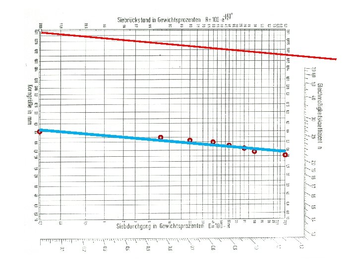
 – The Rosin Rammler Sperling Bennet (RRSB)-function in double ln-ln")
MUO (size distribution analysis) – The Rosin Rammler Sperling Bennet (RRSB)-function in double ln-ln coordinates

n=2 . 05 0. 53 63% Solomon Bogale Chemical Eng'g Department
")
Assignment – The particle size distribution of a powder (density = 2650 kg/m 3) has been determined using a serious of sieves. Calculate the average diameter. Calculate the area and volume distribution. Compare which analytical function describes it well. under size Mass fraction Sieve Opening (mm) 0 0. 4 7 0. 56 20 0. 66 30 0. 68 47 0. 72 58 0. 74 74 0. 78 85 0. 80 100 0. 90
- Slides: 59