Multiway Data Analysis Johan Westerhuis Biosystems Data Analysis

Multiway Data Analysis Johan Westerhuis Biosystems Data Analysis Swammerdam Institute for Life Sciences Universiteit van Amsterdam

The “future” science faculty of the Universiteit van Amsterdam

The Biosystems Data Analysis group officially started in 2004 as a follow up of the process analysis group at the Universiteit van Amsterdam. Its aims are: Developing and validation of new data analysis methods for summarizing and visualizing complex structured biological data (Metabolomics / Proteomics).

l Three-way Data l Three-way Models l Three-way Applications

Three-way Data

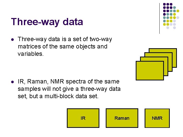
Three-way data l Three-way data is a set of two-way matrices of the same objects and variables. l IR, Raman, NMR spectra of the samples will not give a three-way data set, but a multi-block data set. IR Raman NMR

V U Fluorescence Excitation Sensory Analysis Attributes Image R G B Products J ud ge s Process variables Image Analysis Image Samples Batch Process Samples E Batches m Ti is m si e on Examples of three-way data Chromato graphy Chromatogram

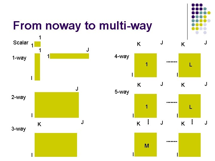
From noway to multi-way Scalar 1 1 -way J 1 J K 4 -way 1 L I I I J K J 1 I 3 -way L I I J J K K M I J K 5 -way 2 -way K J K I I J

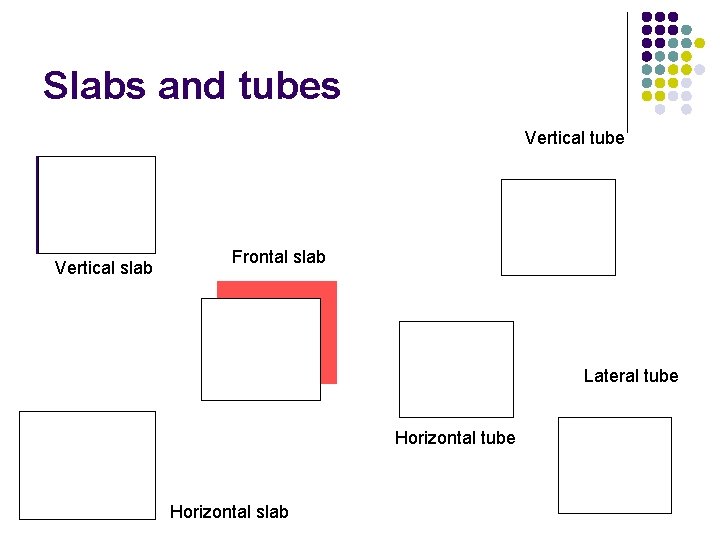
Slabs and tubes Vertical tube Vertical slab Frontal slab Lateral tube Horizontal slab

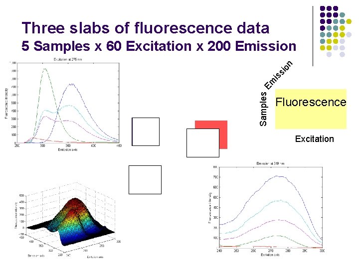
Three slabs of fluorescence data Samples E m is si on 5 Samples x 60 Excitation x 200 Emission Fluorescence Excitation

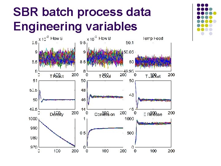
Three-way batch process data l l ‘Engineering’ process data i. e. temperature, pressure, flow rate Spectroscopic process data i. e. NIR, Raman, UV-Vis time batch process variable time process variable One batch X (J K) A series of batches X (I J K)

SBR batch process data Engineering variables

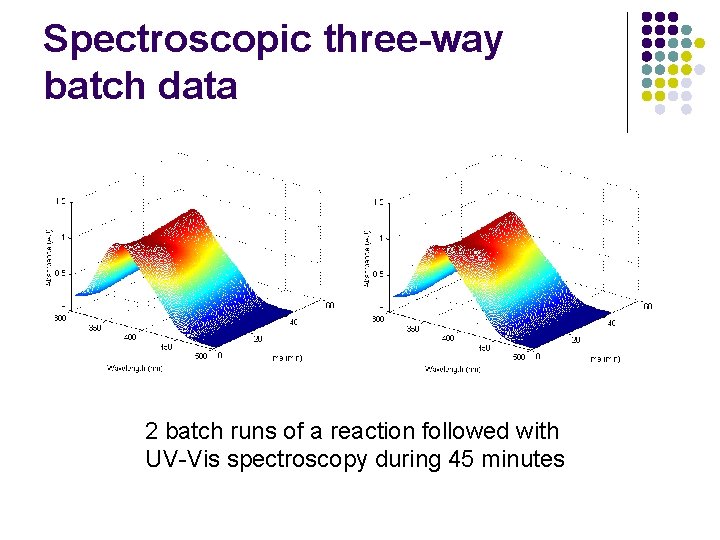
Spectroscopic three-way batch data 2 batch runs of a reaction followed with UV-Vis spectroscopy during 45 minutes

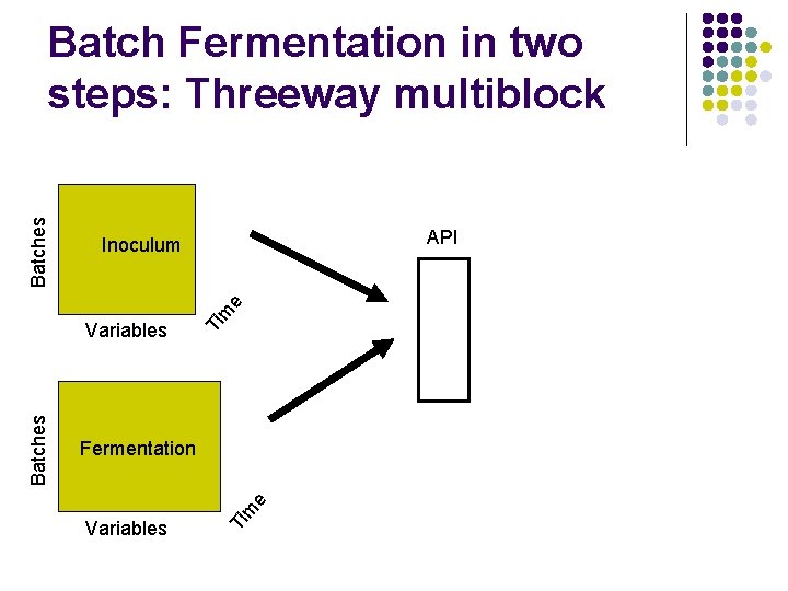
API Inoculum Ti Variables m e Fermentation Ti Batches Variables m e Batches Batch Fermentation in two steps: Threeway multiblock

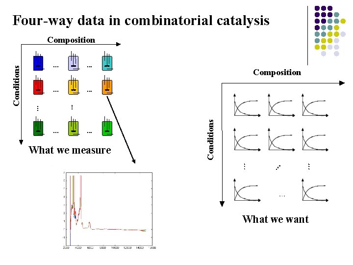
Four-way data in combinatorial catalysis. . . Composition . . . What we measure Conditions . . . Conditions Composition What we want

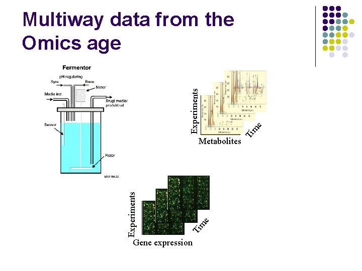
m e Ti Experiments Metabolites Gene expression e m Ti Experiments Multiway data from the Omics age

Three-way Models

Some history M. C. Escher: Small problem with orthogonality

More history l Psychometrics (1944 -1980) l l l Catell 1944: Parallel Proportional profiles (Common factors fitted simultaneously to many data matrices). Tucker 1964: Tucker models Carroll & Chang 1970: Canonical Decomposition (CANDECOMP) Harshman 1970: Parallel Factor Analysis (PARAFAC) Chemistry l l Ho 1978: Rank Annihilation (close to Parafac) on fluorescence data. End 80’s beginning 90’s: Threeway methods to resolve LC -UV data.

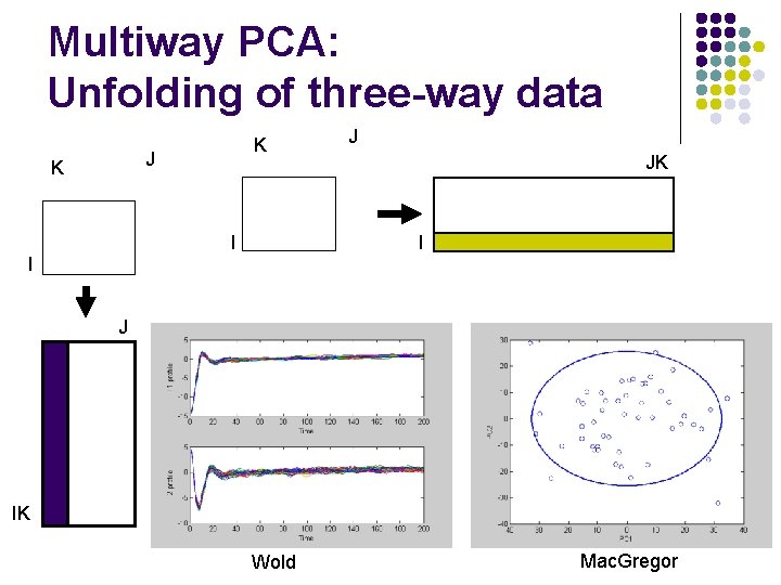
Multiway PCA: Unfolding of three-way data K J K I J JK I I J IK Wold Mac. Gregor

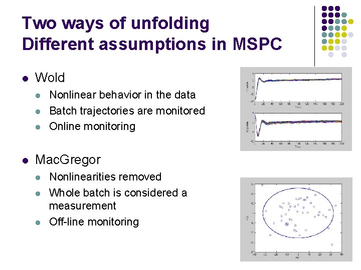
Two ways of unfolding Different assumptions in MSPC l Wold l l Nonlinear behavior in the data Batch trajectories are monitored Online monitoring Mac. Gregor l l l Nonlinearities removed Whole batch is considered a measurement Off-line monitoring

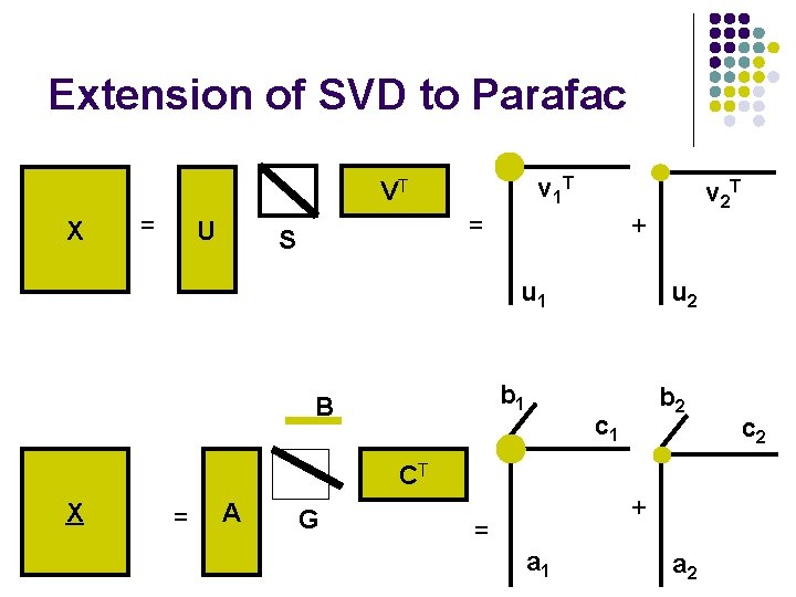
Extension of SVD to Parafac v 1 T VT X = U = S + u 1 b 1 B v 2 T u 2 b 2 c 1 CT X = A G + = a 1 a 2 c 2

Parafac / Candecomp l Parafac is not sequential l l Need to re-estimate whole model when more components are calculated [no deflation]. Parafac solution is unique l l l No rotational freedom Changing parameters will reduce the fit. NB! A PCA model is not unique X = T*PT + E = T*R*R-1*PT + E = C*ST + E Unique ≠ true

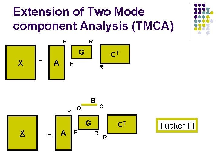
Extension of Two Mode component Analysis (TMCA) P R G X = A CT P R B P Q Q G X = A P CT R R Tucker III

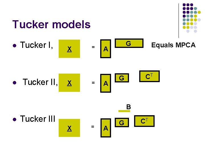
Tucker models l l Tucker I, Tucker II, X X = = G A A Equals MPCA CT G B l Tucker III X = A G CT

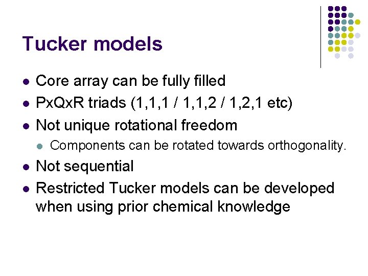
Tucker models l l l Core array can be fully filled Px. Qx. R triads (1, 1, 1 / 1, 1, 2 / 1, 2, 1 etc) Not unique rotational freedom l l l Components can be rotated towards orthogonality. Not sequential Restricted Tucker models can be developed when using prior chemical knowledge

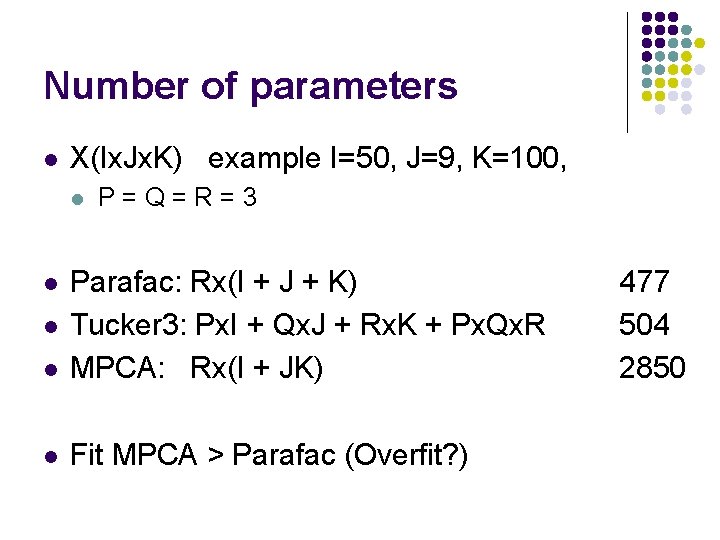
Number of parameters l X(Ix. Jx. K) example I=50, J=9, K=100, l P=Q=R=3 l Parafac: Rx(I + J + K) Tucker 3: Px. I + Qx. J + Rx. K + Px. Qx. R MPCA: Rx(I + JK) l Fit MPCA > Parafac (Overfit? ) l l 477 504 2850

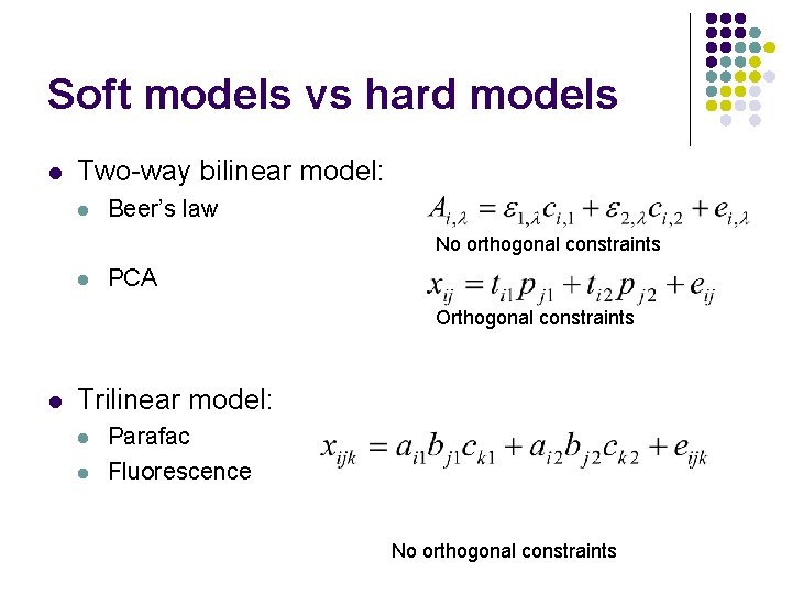
Soft models vs hard models l Two-way bilinear model: l Beer’s law No orthogonal constraints l PCA Orthogonal constraints l Trilinear model: l l Parafac Fluorescence No orthogonal constraints

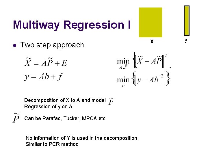
Multiway Regression I l Two step approach: Decomposition of X to A and model Regression of y on A Can be Parafac, Tucker, MPCA etc No information of Y is used in the decomposition Similar to PCR method X y. Y

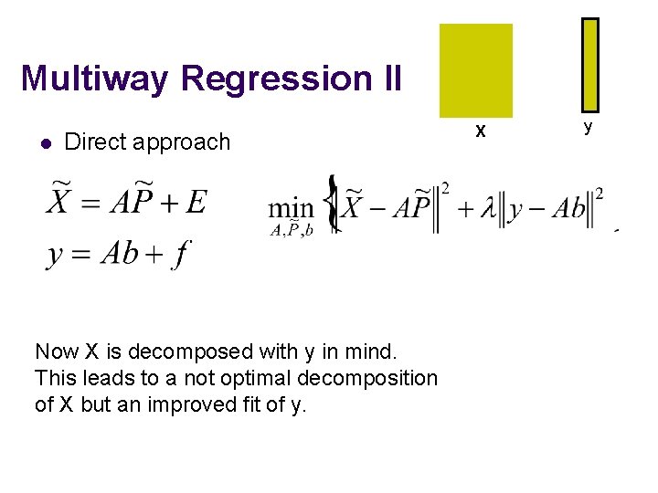
Multiway Regression II l Direct approach Now X is decomposed with y in mind. This leads to a not optimal decomposition of X but an improved fit of y. X y. Y

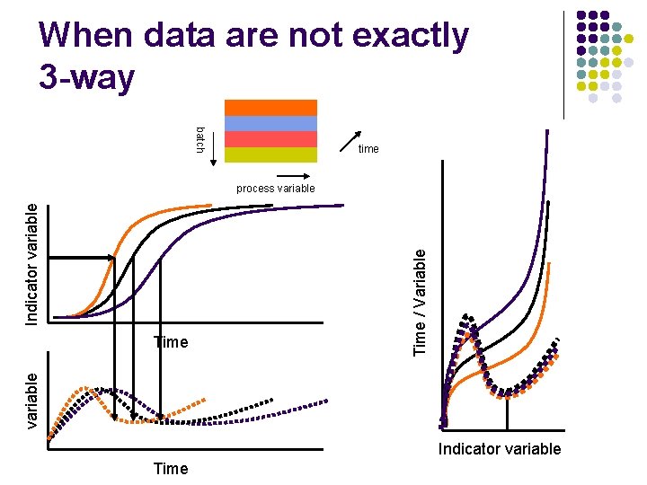
When data are not exactly 3 -way batch time variable Time / Variable Indicator variable process variable Indicator variable Time

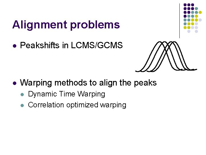
Alignment problems l Peakshifts in LCMS/GCMS l Warping methods to align the peaks l l Dynamic Time Warping Correlation optimized warping

Three-way Applications

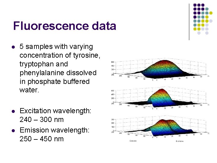
Fluorescence data l 5 samples with varying concentration of tyrosine, tryptophan and phenylalanine dissolved in phosphate buffered water. l Excitation wavelength: 240 – 300 nm Emission wavelength: 250 – 450 nm l

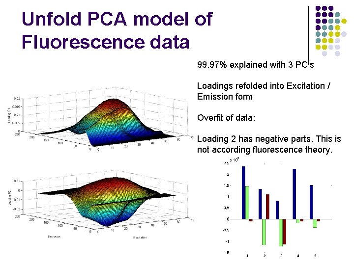
Unfold PCA model of Fluorescence data 99. 97% explained with 3 PC’s Loadings refolded into Excitation / Emission form Overfit of data: Loading 2 has negative parts. This is not according fluorescence theory.

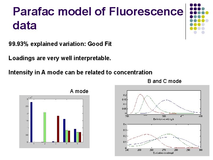
Parafac model of Fluorescence data 99. 93% explained variation: Good Fit Loadings are very well interpretable. Intensity in A mode can be related to concentration B and C mode A mode

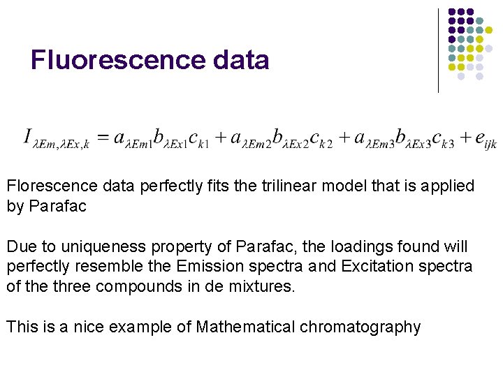
Fluorescence data Florescence data perfectly fits the trilinear model that is applied by Parafac Due to uniqueness property of Parafac, the loadings found will perfectly resemble the Emission spectra and Excitation spectra of the three compounds in de mixtures. This is a nice example of Mathematical chromatography

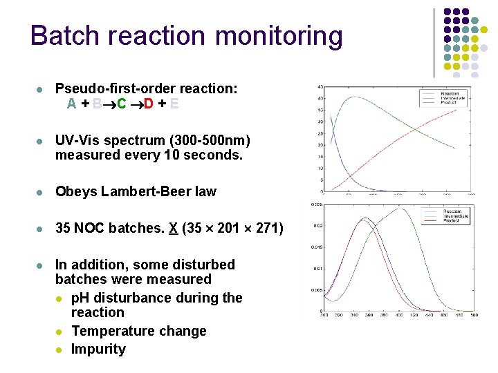
Batch reaction monitoring l Pseudo-first-order reaction: A + B C D + E l UV-Vis spectrum (300 -500 nm) measured every 10 seconds. l Obeys Lambert-Beer law l 35 NOC batches. X (35 201 271) l In addition, some disturbed batches were measured l p. H disturbance during the reaction l Temperature change l Impurity

Aims and goals of research I l Data modelling: l l Analysis of historical batches: l l Improve understanding of process by interpretation of model parameters Are the current process measurements able to distinguish between ‘good’ and ‘bad’ batches? On-line monitoring: l l l Rapid fault detection Easier fault diagnosis: what is the cause of the fault? Prediction of batch duration

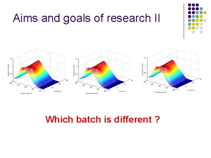
Aims and goals of research II Which batch is different ?

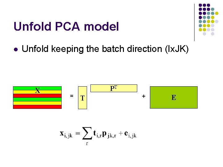
Unfold PCA model l Unfold keeping the batch direction (Ix. JK) X PT = T + E

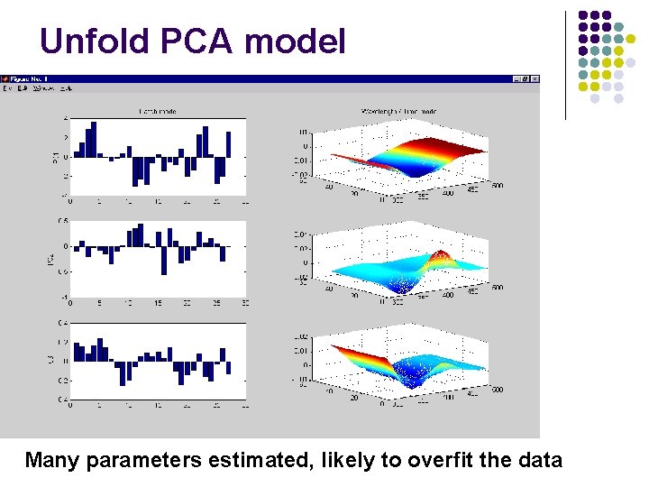
Unfold PCA model Many parameters estimated, likely to overfit the data

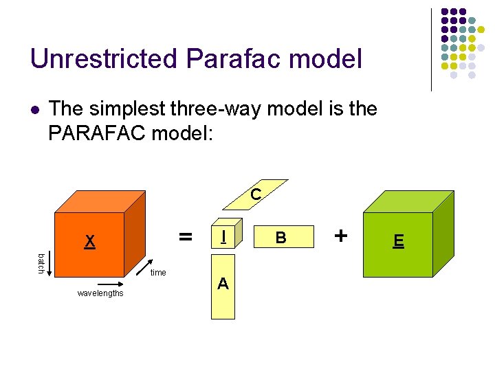
Unrestricted Parafac model l The simplest three-way model is the PARAFAC model: C = X batch time wavelengths I A B + E

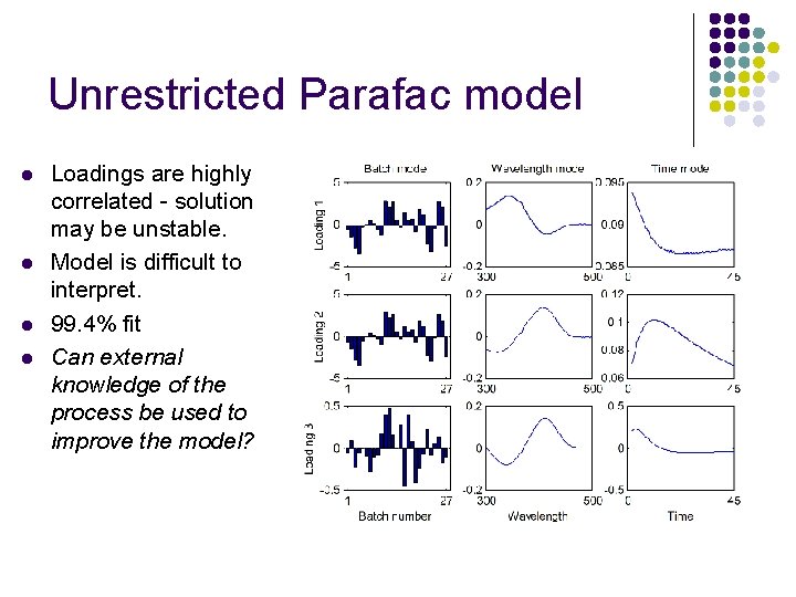
Unrestricted Parafac model l l Loadings are highly correlated - solution may be unstable. Model is difficult to interpret. 99. 4% fit Can external knowledge of the process be used to improve the model?

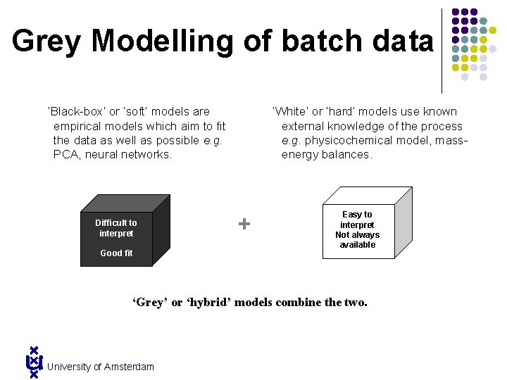
Grey Modelling of batch data ‘Black-box’ or ‘soft’ models are empirical models which aim to fit the data as well as possible e. g. PCA, neural networks. Difficult to interpret Good fit ‘White’ or ‘hard’ models use known external knowledge of the process e. g. physicochemical model, massenergy balances. + Easy to interpret Not always available Good fit ‘Grey’ or ‘hybrid’ models combine the two. University of Amsterdam

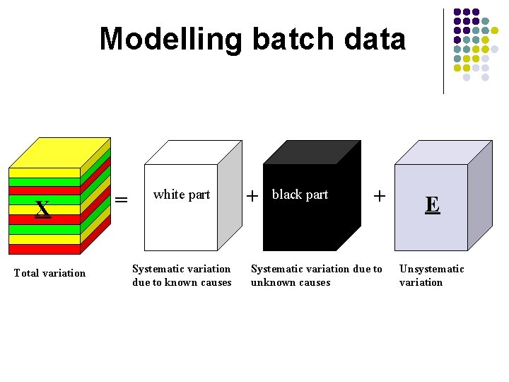
Modelling batch data X Total variation = white part Systematic variation due to known causes + black part + Systematic variation due to unknown causes E Unsystematic variation

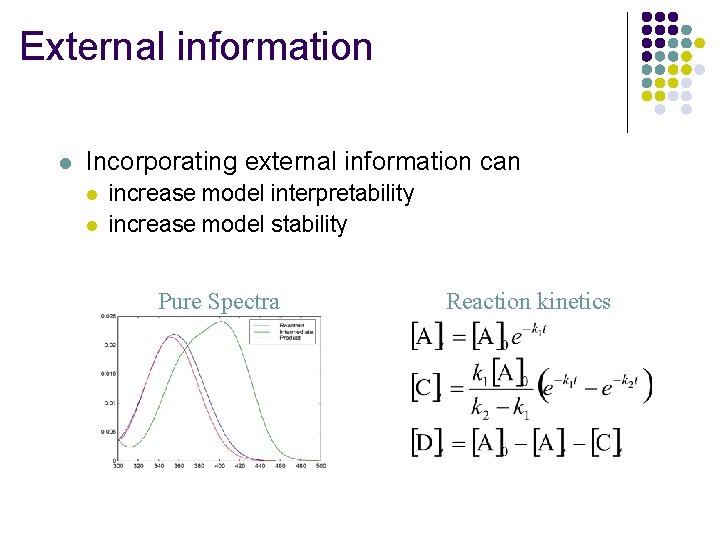
External information l Incorporating external information can l l increase model interpretability increase model stability Pure Spectra Reaction kinetics

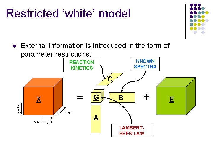
Restricted ‘white’ model l External information is introduced in the form of parameter restrictions: KNOWN SPECTRA REACTION KINETICS C = X batch time wavelengths G B + A LAMBERTBEER LAW E

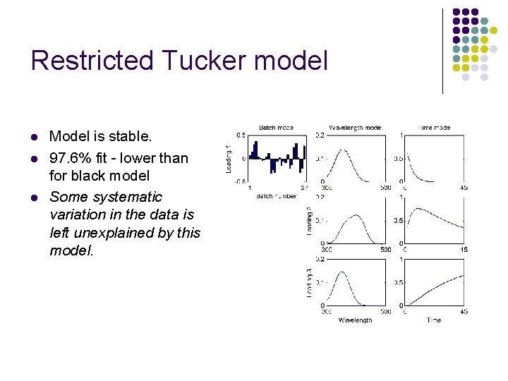
Restricted Tucker model l Model is stable. 97. 6% fit - lower than for black model Some systematic variation in the data is left unexplained by this model.

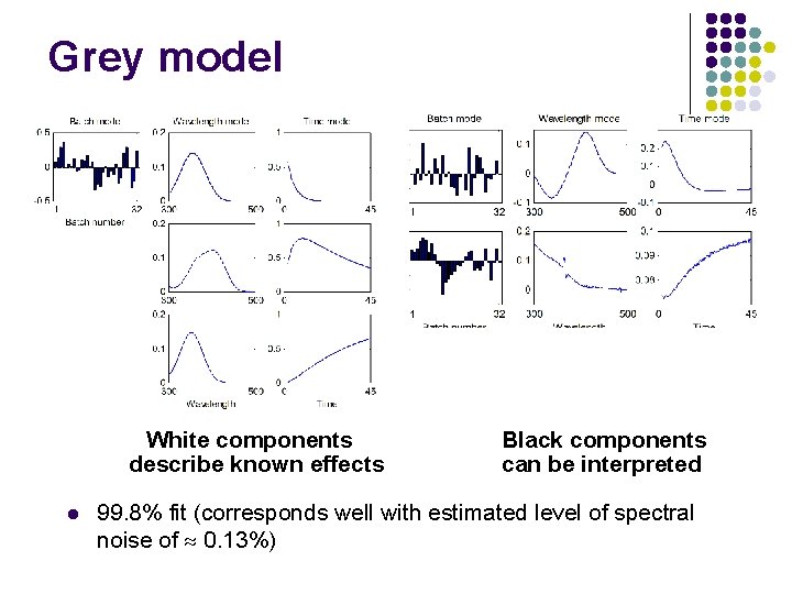
Grey model White components describe known effects l Black components can be interpreted 99. 8% fit (corresponds well with estimated level of spectral noise of 0. 13%)

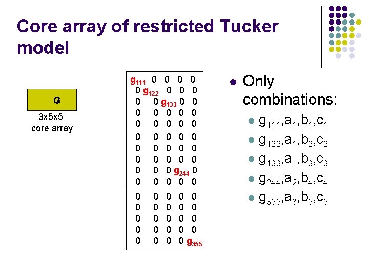
Core array of restricted Tucker model G 3 x 5 x 5 core array g 111 0 0 0 g 122 0 0 0 g 133 0 0 0 0 0 0 0 0 g 244 0 0 0 0 0 0 0 0 g 355 l Only combinations: l l l g 111, a 1, b 1, c 1 g 122, a 1, b 2, c 2 g 133, a 1, b 3, c 3 g 244, a 2, b 4, c 4 g 355, a 3, b 5, c 5

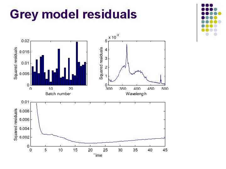
Grey model residuals

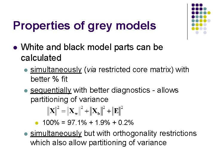
Properties of grey models l White and black model parts can be calculated l l simultaneously (via restricted core matrix) with better % fit sequentially with better diagnostics - allows partitioning of variance l l 100% = 97. 1% + 1. 9% + 0. 2% simultaneously but with orthogonality restrictions which also allow partitioning of variance

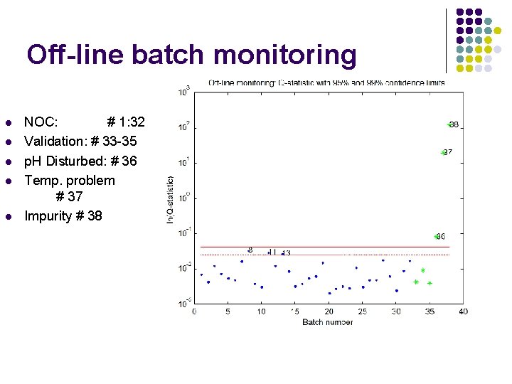
Off-line batch monitoring l l l NOC: # 1: 32 Validation: # 33 -35 p. H Disturbed: # 36 Temp. problem # 37 Impurity # 38

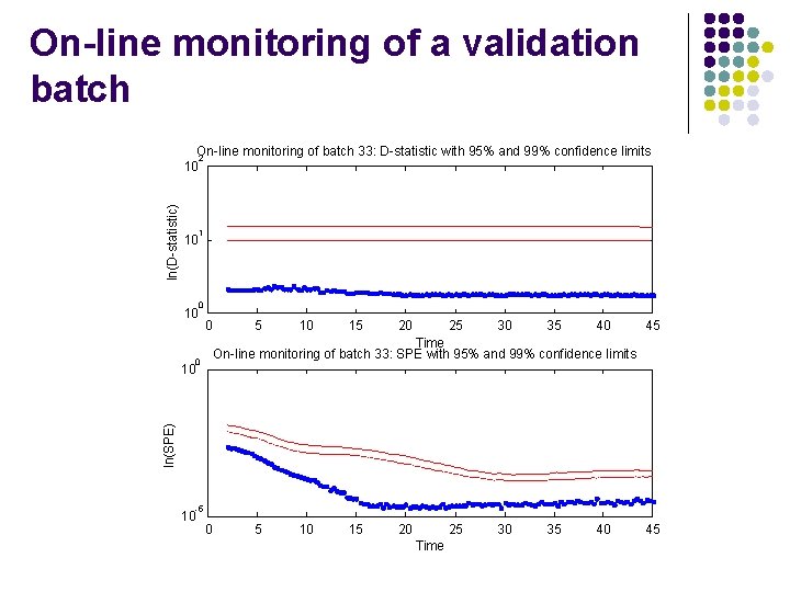
On-line monitoring of a validation batch ln(D-statistic) On-line monitoring of batch 33: D-statistic with 95% and 99% confidence limits 2 10 1 10 0 5 10 15 20 25 30 35 40 45 Time On-line monitoring of batch 33: SPE with 95% and 99% confidence limits 0 ln(SPE) 10 -5 10 0 5 10 15 20 25 Time 30 35 40 45

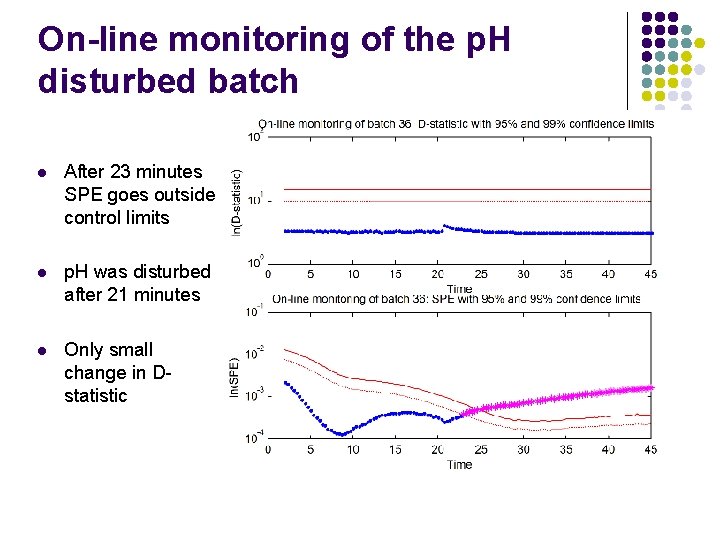
On-line monitoring of the p. H disturbed batch l After 23 minutes SPE goes outside control limits l p. H was disturbed after 21 minutes l Only small change in Dstatistic

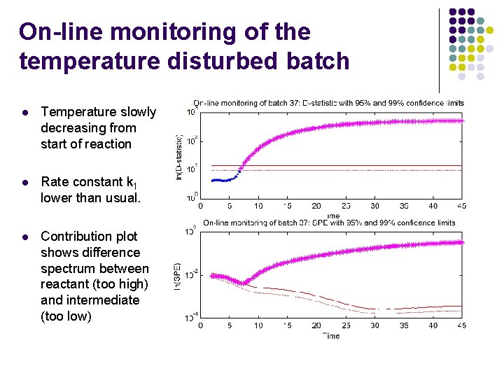
On-line monitoring of the temperature disturbed batch l Temperature slowly decreasing from start of reaction l Rate constant k 1 lower than usual. l Contribution plot shows difference spectrum between reactant (too high) and intermediate (too low)

Want to know more Look at Rasmus Bro’s website