Multivariate QTL Linkage Analysis David M Evans Queensland

Multivariate QTL Linkage Analysis David M. Evans Queensland Institute of Medical Research Brisbane Australia Twin Workshop Boulder 2003

Introduction How best to analyze data from n correlated variables? (1) Run n univariate tests of linkage? (2) -Increased type I error (3) -How to interpret the results? (4) -Doesn’t take advantage of the multivariate structure of the data (5) (2) Multivariate Analysis (6) -Increased Power vs Univariate case (7) -Type I error controlled (8) -Advantages in interpretation: (9) other (10) -See effect of the QTL on each variable in context of all the measures -Less prone to stochastic variation?

Methods (1) Linear Composite techniques (e. g. Amos et al. , 1990) (2) Factor Score Method (Boomsma, 1996) (3) Fitting the full multivariate model to the data (Eaves, Neale & Maes, 1996; Martin, Boomsma & Machin, 1997)

(1) Linear Composites Central idea is to create a linear composite of the multivariate phenotypes, and then to perform the linkage analysis on this composite -e. g. Amos et al. , 1990: Suggested an extension to Haseman-Elston regression: ^ +e (Yi 1 – Yi 2)2 = β 0 + β 1*π i i i. e. Estimate a linear composite of squared pair differences in trait measurements which has the strongest correlation between the proportion of alleles shared IBD at the marker locus: ^ i + ei [α 1(y 11 - y 12) + α 2(y 21 - y 22) +. . . αk(yk 1 - yk 2)]2 = β 0 + β 1*π k with the constraint Σ α = 1. j =1 -e. g. Marlow et al. (2003) Perform a Principle Components Analysis, then analyze first principal component as in a univariate analysis

(1) Linear Composites Problems: -Amos et al. 1990 method has all problems associated with Haseman-Elston -Generalization to complex pedigrees? -Power of approaches relative to fitting the full multivariate model? ?

(2) Factor score method (Boomsma et al. , 1996) Calculate factor scores on a pleiotropic genetic factor and then perform a linkage analysis on these genetic factor scores p = 4 variables 0. 5 m = 2 pleiotropic factors G 1 λ 1 g E 1 λ 4 g G 2 λ 1 g λ 2 g λ 3 g V 11 V 12 V 13 ε 11 ε 12 ε 13 V 14 ε 14 E 2 λ 4 g λ 2 g λ 3 g V 21 V 22 V 23 ε 21 ε 22 ε 23 Vip = λpg. Gi + λpe. Ei + εip V 24 ε 24

(1) Fit a common factor model to the data and estimate factor loadings Σ = ΛΨΛ' + Θ Σ is 2 p x 2 p expected covariance matrix, Λ is 2 p x 2 m matrix of factor loadings Θ is the estimated 2 p x 2 p matrix of unique variances Ψ is the 2 m x 2 m matrix of factor correlations specified apriori 0. 5 p = 4 variables m = 2 pleiotropic factors G 11 λ 1 g E 11 λ 4 g G 21 λ 1 g λ 2 g λ 3 g V 11 V 12 V 13 ε 11 ε 12 ε 13 V 14 ε 14 E 21 λ 4 g λ 2 g λ 3 g V 21 V 22 V 23 ε 21 ε 22 ε 23 V 24 ε 24

Σ is 2 p x 2 p expected covariance matrix, Λ is 2 p x 2 m matrix of factor loadings Θ is the estimated 2 p x 2 p matrix of unique variances Ψ is the 2 m x 2 m matrix of factor correlations (2) Calculate a weight matrix A (Thurstone): A = ΨΛ' Σ-1 A = ΨΛ'(ΛΨΛ' + Θ)-1 Weight matrix is obtained by minimizing the sum of squared differences between estimated and true factor scores. Equivalent to finding the linear regression of factor scores on phenotypes. (3) Estimate the genetic factor scores by premultiplying the matrix of multivariate phenotypes by a weight matrix A: f= A’P

Advantages: -Partitions out environmental and background genetic noise -Selective genotyping of subjects Disadvantage: -The weight matrix used to calculate the factor scores is calculated from the sample as the actual factor scores- i. e. the information used to calculate the weight matrix and the information used to test for linkage are not independent

(3) Fitting the Full Multivariate Model ^ π Q 21 Q 1 q 1 P 11 q 2 q 3 P 12 P 13 q 1 P 21 q 2 P 22 QTL is parameterized as a latent factor which pleiotropically affects the phenotypes of interest ^ Correlation between QTL factors is set as π NB. QTL within twin cross-trait covariance is the square root of the product of the qtl variances. q 3 P 23

^ π Q 21 Q 1 q 2 P 11 a 11 q 3 a 21 P 13 a 11 a 23 A 12 e 21 e 22 E 11 E 12 e 23 a 21 a 33 A 23 0. 5 e 11 e 33 E 13 a 23 A 22 A 21 0. 5 P 23 a 31 a 22 A 13 e 31 q 3 P 22 a 33 0. 5 e 11 q 2 P 21 a 31 a 22 A 11 q 1 e 21 e 31 e 22 E 21 E 22 e 23 e 33 E 23

a 11 Q’ = [q 1, q 2, q 3] A= a 21 a 22 a 31 a 32 a 33 Σ= (6 x 6) e 11 E = e 21 e 22 e 31 e 32 e 33 AA’ + EE’ + QQ’ (0. 5 x AA’) + πi. QQ’ AA’ + EE’ + QQ’

Q 1 q 2 ζa 1 βa 2 A 1 P 2 βc 2 C 1 ζc 1 λe 1 E 1 ζe 1 λa 3 ε 3 P 3 λc 2 λc 1 βc 3 C 2 ζc 2 λe 2 βe 2 E 2 ζe 2 ζa 3 A 3 λa 2 ε 2 P 1 βa 3 A 2 λa 1 ε 1 q 3 ζa 2 C 3 λe 3 βe 3 E 3 ζe 3 ζc 3

“Pi hat” method -The likelihood for each pedigree (i) is calculated as: L(θ) = (2π-k)|Σi|-1/2 exp[-1/2(yi - μ)’Σi-1(yi - μ)] -where Σi = AA’ + EE’ + QQ’ (0. 5 x AA’) + πi. QQ’ AA’ + EE’ + QQ’ -Easy to specify, especially in large pedigrees, but… -Computationally intensive -Bias in selected samples

“Full IBD Method” -The likelihood for each pedigree (i) is calculated as: P(IBD = 0)(2π-k)|Σ 0|-1/2 exp[-1/2(yi - μ)’Σ 0 -1(yi - μ)] + P(IBD = 1)(2π-k)|Σ 1|-1/2 exp[-1/2(yi - μ)’Σ 1 -1(yi - μ)] + P(IBD = 2)(2π-k)|Σ 2|-1/2 exp[-1/2(yi - μ)’Σ 2 -1(yi - μ)] AA’ + EE’ + QQ’ Σ 0 = (0. 5 x AA’) AA’ + EE’ + QQ’ Σ 1 = (0. 5 x AA’) + 0. 5*QQ’ AA’ + EE’ + QQ’ Σ 2 = (0. 5 x AA’) + QQ’ -Computationally efficient -Difficult to specify in large sibships/pedigrees AA’ + EE’ + QQ’

Likelihood Ratio Test Under standard conditions, twice the difference in natural log-likelihood between models is distributed asymptotically as a χ2 distribution with degrees of freedom equal to the difference in the number of parameters between the models BUT In linkage analysis, the likelihood ratio test is conducted under non-standard conditions That is, the true value of some of the parameters under the null hypothesis (i. e. σq 2 = 0) are located on the boundary of the parameter space defined by the alternative hypothesis. Under these conditions, the likelihood ratio statistic is distributed as a mixture of χ 2 distributions, with the mixing proportions determined by the geometry of the parameter space. For example, in the case of a univariate VC linkage analysis, the test is asymptotically distributed as a 50: 50 mixture of χ12 and a point mass at zero (Self & Liang, 1987).

Likelihood Ratio Test In multivariate tests of linkage, the situation is even more complicated and determining the asymptotic distribution of the test statistic is difficult. For example, in the case of a bivariate test for linkage, Amos et al. (2002) suggests that the test for linkage is distributed asymptotically as: ¼ χ02 : ½χ12 : ¼χ22 Therefore evaluating the test against χ22 will result in a conservative test- although as the number of variables increases, this difference may become small (Marlow et al. , 2003). Perhaps the best strategy at the present time is to evaluate significance using empirically derived significance values.

Why is power increased? ^π Q 1 Q 2 q 1 V V Sib One Sib Two Σ = q 12 ^ πq 12

Why is power increased? ^π Q 1 Q 2 q 1 q 2 V 11 q 1 V 12 q 2 V 21 Sib One V 22 Sib Two q 12 Σ = q 1 q 2 q 22 ^ πq 1 q 2 q 12 ^ πq 1 q 2 ^ πq 22 q 1 q 2 q 22

Under what Conditions is Power Greatest? ^π Q q 1 Q q 2 β E 1 q 1 E 2 e 1 E 1 e 2 V 11 α s 1 S 1 E 2 e 1 V 12 e 2 V 21 s 2 S 2 V 22 α s 1 α q 2 β S 1 s 2 -q 1 and q 2 large S 2 -s 1 and s 2 are large 1 1 α Sibling One Sibling Two -QTL and residual sources of covariation operate in opposite directions

(q 1 = q 2 = 20%; s 1 = s 2 = 40%; e 1 = e 2 = 40%) Power depends on direction and source of residual phenotypic correlation

Implications -One is most likely to detect a QTL that induces a correlation between variables in the opposite direction to the residual correlation => variables with low phenotypic correlations -Therefore a simple inspection of correlation matrices may not reveal which combination of variables would be best to combine in a multivariate analysis. Perhaps the decision is best guided by information on the biological system being considered. -Can this fact be taken advantage of experimentally?

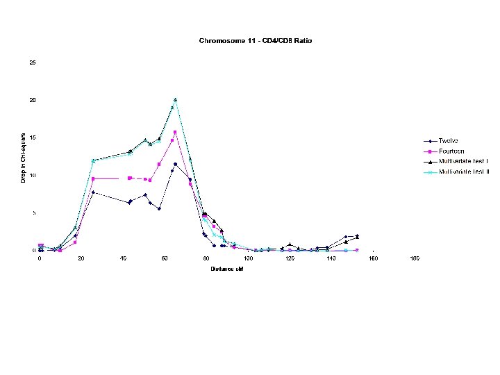
Example CD 4/CD 8 ratio Project: -Australian monozygotic and dizygotic twins bled at twelve, fourteen and sixteen years of age. -Measured longitudinally on a variety of hematological and immunological indices, including CD 4/CD 8 ratio which is a measure of immune function Significance: -CD 4/CD 8 ratio is depressed in a variety of conditions including AIDS, Graft-versus Host disease, and some viral infections -CD 4/CD 8 ratio predicts the course of HIV infection -Localising a QTL for CD 4/CD 8 ratio is of therapeutic significance

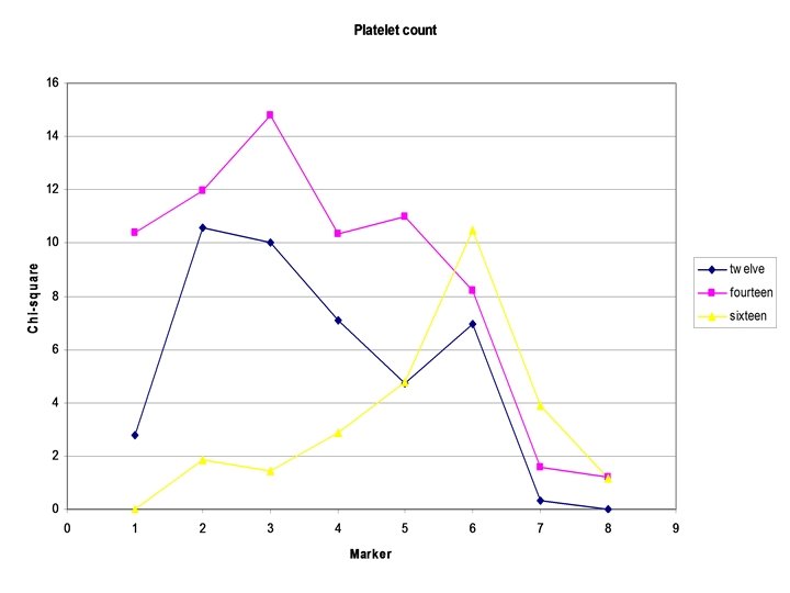
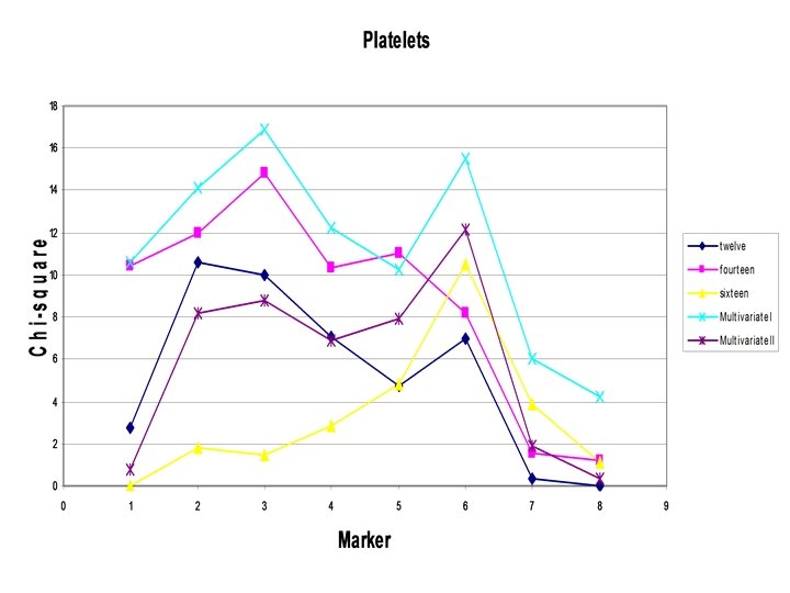
Example: Platelet count

Q 1 q 2 ζa 1 βa 2 A 1 βd 2 ζd 1 1 ζe 1 ε 3 P 3 1 1 1 D 1 1 P 2 ε 2 βd 3 D 2 ζd 2 1 βe 2 E 2 ζe 2 ζa 3 A 3 1 P 1 E 1 βa 3 A 2 1 ε 1 q 3 ζa 2 D 3 1 βe 3 E 3 ζe 3 ζ -Variance of the innovations are estimated λ - Factor loadings are constrained to unity ζd 3

The residual structures can be expressed compactly in matrix algebra form e. g. : A = (I - B)-1 * Ψ * (I - B)-1 ’ + Θε I is an identity matrix B is the matrix of transmission coefficients B= 0 0 0 β 2 0 0 0 β 3 0 var(ζ 1 a) Ψ is the matrix of innovation variances Ψ= 0 0 0 var(ζ 2 a) 0 0 0 var(ζ 3 a)

Mx Script Platelet count

Issues: -Has the method increased power? ? ? If not why? -Equating factor loadings? -Likelihood of base model?