Multivariate Probability Distributions Lecture 17 Chapter 7 Study
Multivariate Probability Distributions Lecture 17 • • • Chapter 7 – Study this closely Chapter 16 Sections 3. 9. 1 -3. 9. 7 and 4. 3 Lecture 17 Multivariate Empirical Dist. xlsx Lecture 17 Multivariate Normal Dist. xlsx Lecture 17 Correct Std Dev EMP. xlsx

Multivariate Probability Distributions • Multivariate (MV) Distribution --Two or more random variables that are correlated – Can be MV Normal – Or MV EMP – Or MV Beta – Or MV Mixed (Normal for X 1 and EMP for X 2) • We have been working with univariate distributions, now we have many distributions and they are assumed to be correlated to one another
Parameter Estimation for MV Dist. • Data are generated contemporaneously – Price and yield are observed each year for related commodities • Corn and sorghum used interchangeably for animal feed so prices are related • Steer and heifer prices are related • Yields of crops on the same farm have the same weather conditions – Supply and demand forces affect prices similarly, bear market or bull market; prices move together • Prices for tech stocks move together • Prices for an industry or sector’s stocks move together
Why go to the Extra Effort for MV? • If correlation is ignored when random variables are correlated, results are biased: ~ ~ • If Z = Ỹ 1 + Ỹ 2 OR Z = Ỹ 1 * Ỹ 2 and the model is simulated without correlation, so ρ1, 2 =0 – But the true ρ1, 2 > 0 then the model will ~ understate the risk for Z – But the true ρ1, 2 < 0 then the model will ~ overstate the risk for Z ~ • If Z = Ỹ 1 * Ỹ 2 – The Mean of Z is biased, as well
Different MV Distributions • Multivariate Normal distribution – MVN • Multivariate Empirical – MVE • Multivariate Mixed where each variable is distributed differently, such as, a MV Mixed distribution with five variables: – X ~ Uniform, – Y ~ Normal, – Z ~ Empirical, – R ~ Beta, and – S ~ Gamma
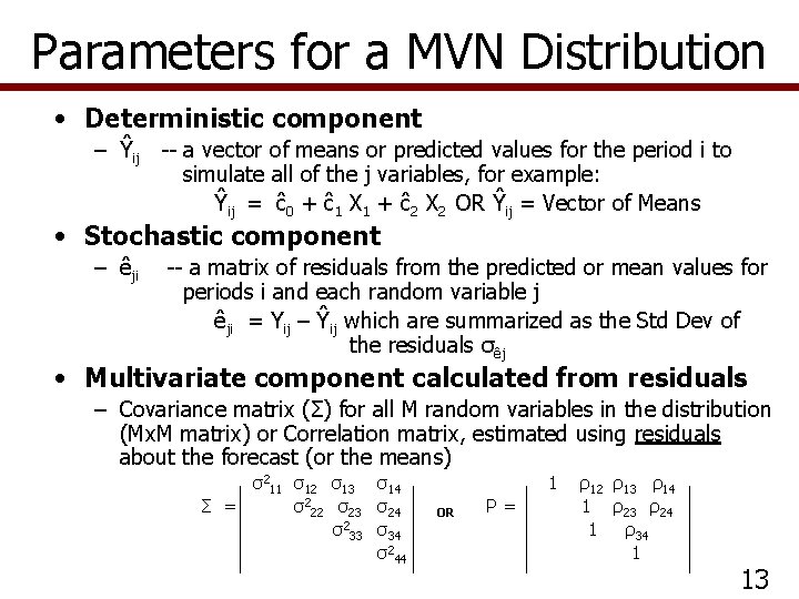
Parameters for a MVN Distribution • Deterministic component – Ŷij -- a vector of means or predicted values for the period i to simulate all of the j variables, for example: Ŷij = ĉ0 + ĉ1 X 1 + ĉ2 X 2 OR Ŷij = Vector of Means • Stochastic component – êji -- a matrix of residuals from the predicted or mean values for periods i and each random variable j êji = Yij – Ŷij which are summarized as the Std Dev of the residuals σêj • Multivariate component calculated from residuals – Covariance matrix (Σ) for all M random variables in the distribution (Mx. M matrix) or Correlation matrix, estimated using residuals about the forecast (or the means) σ211 σ12 σ13 σ14 Σ = σ222 σ23 σ24 σ233 σ34 σ244 1 OR Ρ= ρ12 ρ13 ρ14 1 ρ23 ρ24 1 ρ34 1 13

Three Variable MVN Distribution • Deterministic component for three random variables – Ĉi = a + b 1 Ci-1 – Ŵi = a + b 1 Ti + b 2 Wi-1 – Ŝi = a + b 1 T i • Stochastic component – êCi = Ci – Ĉi – êWi = Wi – Ŵi – êSi = Si – Ŝi • Multivariate component calculated from the residuals σ2 cc σcw σcs Σ = σ2 ww σws OR P= σ2 ss
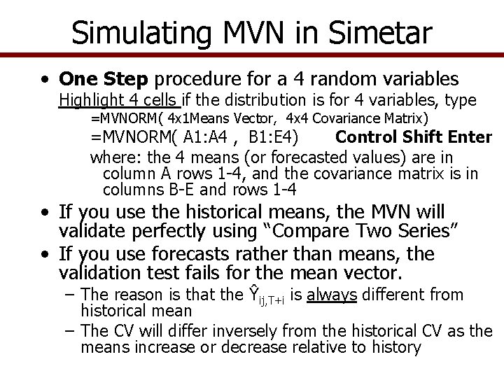
Simulating MVN in Simetar • One Step procedure for a 4 random variables Highlight 4 cells if the distribution is for 4 variables, type =MVNORM( 4 x 1 Means Vector, 4 x 4 Covariance Matrix) =MVNORM( A 1: A 4 , B 1: E 4) Control Shift Enter where: the 4 means (or forecasted values) are in column A rows 1 -4, and the covariance matrix is in columns B-E and rows 1 -4 • If you use the historical means, the MVN will validate perfectly using “Compare Two Series” • If you use forecasts rather than means, the validation test fails for the mean vector. – The reason is that the Ŷij, T+i is always different from historical mean – The CV will differ inversely from the historical CV as the means increase or decrease relative to history
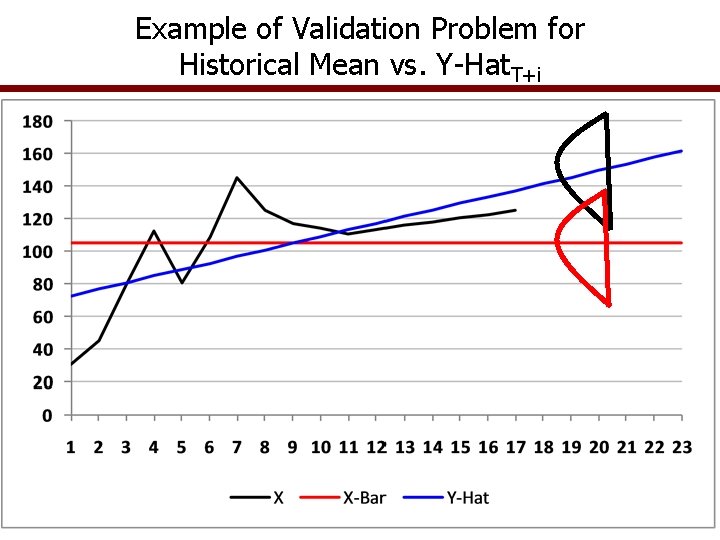
Example of Validation Problem for Historical Mean vs. Y-Hat. T+i
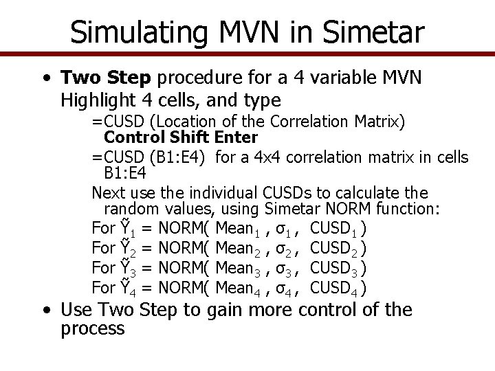
Simulating MVN in Simetar • Two Step procedure for a 4 variable MVN Highlight 4 cells, and type =CUSD (Location of the Correlation Matrix) Control Shift Enter =CUSD (B 1: E 4) for a 4 x 4 correlation matrix in cells B 1: E 4 Next use the individual CUSDs to calculate the random values, using Simetar NORM function: For Ỹ 1 = NORM( Mean 1 , σ1 , CUSD 1 ) For Ỹ 2 = NORM( Mean 2 , σ2 , CUSD 2 ) For Ỹ 3 = NORM( Mean 3 , σ3 , CUSD 3 ) For Ỹ 4 = NORM( Mean 4 , σ4 , CUSD 4 ) • Use Two Step to gain more control of the process
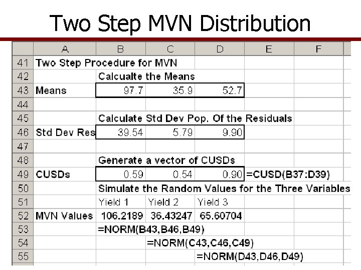
Two Step MVN Distribution
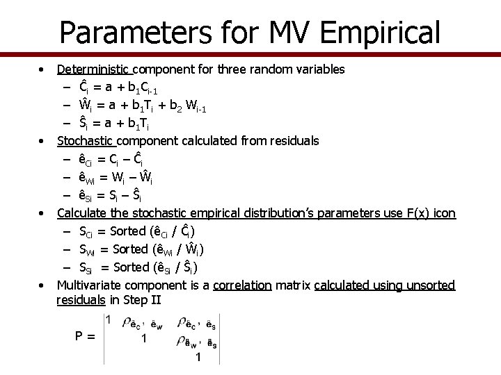
Parameters for MV Empirical • • Deterministic component for three random variables – Ĉi = a + b 1 Ci-1 – Ŵi = a + b 1 Ti + b 2 Wi-1 – Ŝi = a + b 1 T i Stochastic component calculated from residuals – êCi = Ci – Ĉi – êWi = Wi – Ŵi – êSi = Si – Ŝi Calculate the stochastic empirical distribution’s parameters use F(x) icon – SCi = Sorted (êCi / Ĉi) – SWi = Sorted (êWi / Ŵi) – SSi = Sorted (êSi / Ŝi) Multivariate component is a correlation matrix calculated using unsorted residuals in Step II P=
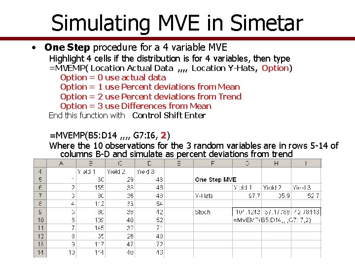
Simulating MVE in Simetar • One Step procedure for a 4 variable MVE Highlight 4 cells if the distribution is for 4 variables, then type =MVEMP( Location Actual Data , , Location Y-Hats, Option) Option = 0 use actual data Option = 1 use Percent deviations from Mean Option = 2 use Percent deviations from Trend Option = 3 use Differences from Mean End this function with Control Shift Enter =MVEMP(B 5: D 14 , , G 7: I 6, 2) Where the 10 observations for the 3 random variables are in rows 5 -14 of columns B-D and simulate as percent deviations from trend
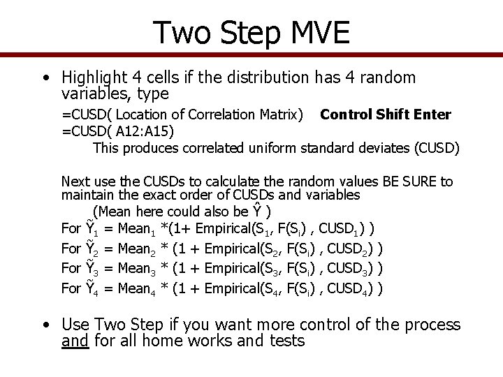
Two Step MVE • Highlight 4 cells if the distribution has 4 random variables, type =CUSD( Location of Correlation Matrix) Control Shift Enter =CUSD( A 12: A 15) This produces correlated uniform standard deviates (CUSD) Next use the CUSDs to calculate the random values BE SURE to maintain the exact order of CUSDs and variables (Mean here could also be Ŷ ) For Ỹ 1 = Mean 1 *(1+ Empirical(S 1, F(Si) , CUSD 1) ) For Ỹ 2 = Mean 2 * (1 + Empirical(S 2, F(Si) , CUSD 2) ) For Ỹ 3 = Mean 3 * (1 + Empirical(S 3, F(Si) , CUSD 3) ) For Ỹ 4 = Mean 4 * (1 + Empirical(S 4, F(Si) , CUSD 4) ) • Use Two Step if you want more control of the process and for all home works and tests
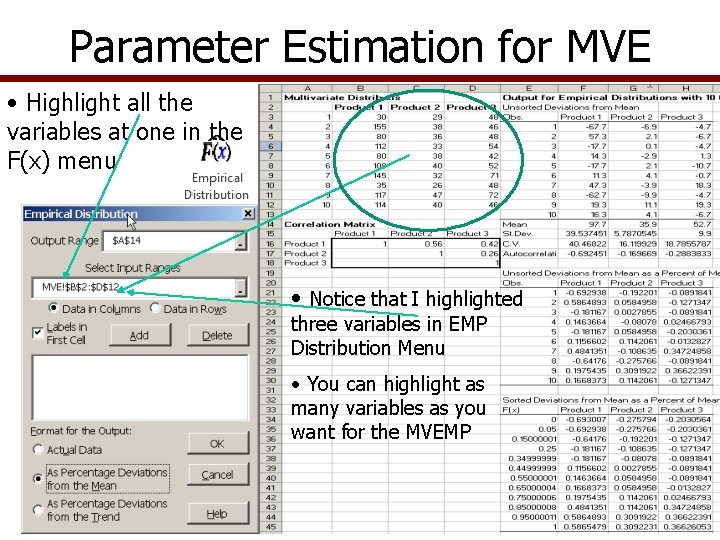
Parameter Estimation for MVE • Highlight all the variables at one in the F(x) menu • Notice that I highlighted three variables in EMP Distribution Menu • You can highlight as many variables as you want for the MVEMP
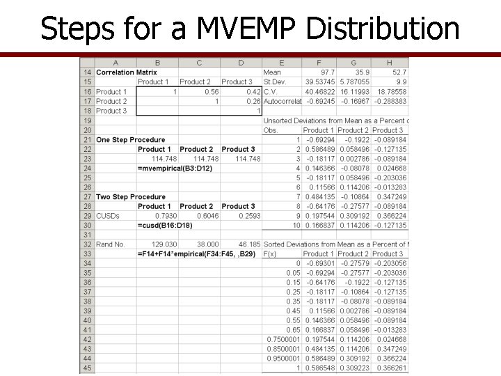
Steps for a MVEMP Distribution
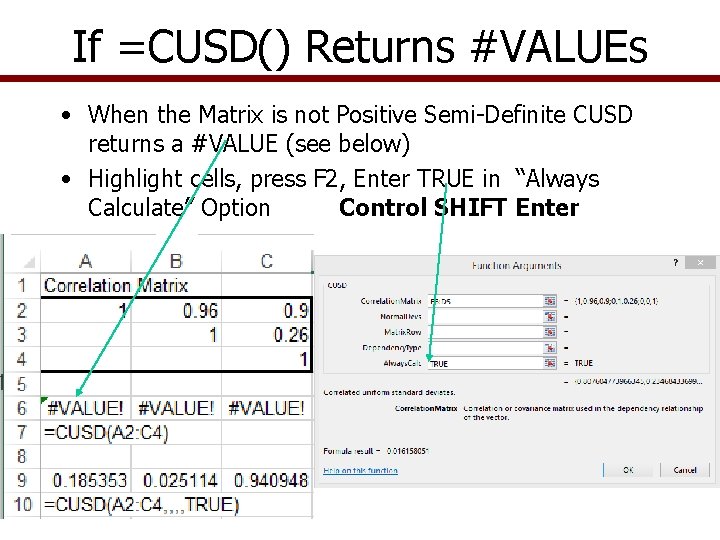
If =CUSD() Returns #VALUEs • When the Matrix is not Positive Semi-Definite CUSD returns a #VALUE (see below) • Highlight cells, press F 2, Enter TRUE in “Always Calculate” Option Control SHIFT Enter
MV Mixed Distributions • What if you need to simulate a MV distribution made up of variables that are not all Normal or all Empirical? For example: – – X is ~ Normal Y is ~ Beta T is ~ Gamma Z is ~ Empirical • Develop parameters for each variable • Estimate the correlation matrix for the random variables in the MV distribution
MV Mixed Distributions • Simulate a vector of Correlated Uniform Standard Deviates using =CUSD() function =CUSD( correlation matrix ) is an array function so highlight the number of cells that matches the number of variables in the MV distribution • Use the CUSDi values in the appropriate Simetar functions for each random variable, as: =NORM(Mean, Std Dev, CUSD 1) =BETAINV(CUSD 2, Alpha, Beta) =GAMMAINV(CUSD 3, P 1, P 2) =Mean*(1+EMP(Si, F(Si), CUSD 4))
Validation of MV Distributions • Simulate the model and specify the random variables as the KOVs, then test the simulated random values • Perform the following tests – Use the Compare Two Series Tab in Ho. Hi to: • Test means and covariance for historical series vs. simulated – Use the Check Correlation Tab to test the correlation matrix used as input for the MV model vs. the implied correlation in the simulated random variables • Null hypothesis (Ho) is: Simulated correlationij = Historical correlation coefficientij • If Null hypothesis is true the calculated t statistics will exceed test statistic for the Student t tests • Use caution on means tests if your forecasted Ŷ is different from the historical Ῡ
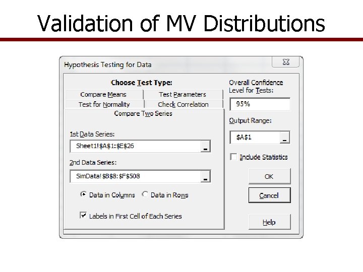
Validation of MV Distributions
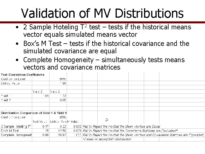
Validation of MV Distributions • 2 Sample Hoteling T 2 test – tests if the historical means vector equals simulated means vector • Box’s M Test – tests if the historical covariance and the simulated covariance are equal • Complete Homogeneity – simultaneously tests means vectors and covariance matrices
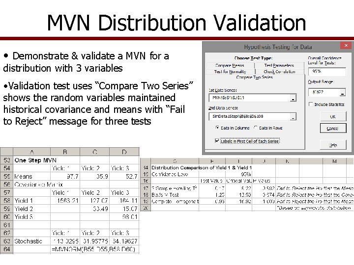
MVN Distribution Validation • Demonstrate & validate a MVN for a distribution with 3 variables • Validation test uses “Compare Two Series” shows the random variables maintained historical covariance and means with “Fail to Reject” message for three tests
- Slides: 23