Multivariate Methods of data analysis Advanced Scientific Computing

Multivariate Methods of data analysis Advanced Scientific Computing Workshop ETH 2014 Helge Voss MAX-PLANCK-INSTITUT FÜR KERNPHYSIK IN HEIDELBERG Helge Voss Advanced Scientific Computing Workshop ETH 2014 1

Overview § Multivariate classification/regression algorithms (MVA) § what they are § how they work § Overview over some classifiers § Multidimensional Likelihood (k. NN : k-Nearest Neighbour) § Projective Likelihood (naïve Bayes) § Linear Classifier § Non linear Classifiers § Neural Networks § Boosted Decision Trees § Support Vector Machines § General comments about: § Overtraining Helge Voss § Systematic errors Advanced Scientific Computing Workshop ETH 2014 2

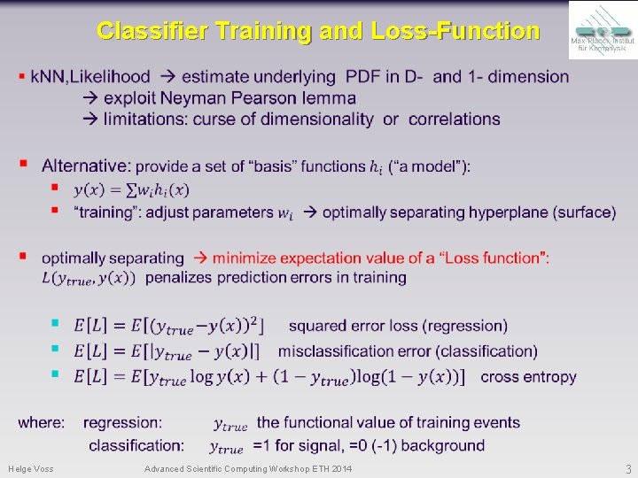
Classifier Training and Loss-Function Helge Voss Advanced Scientific Computing Workshop ETH 2014 3

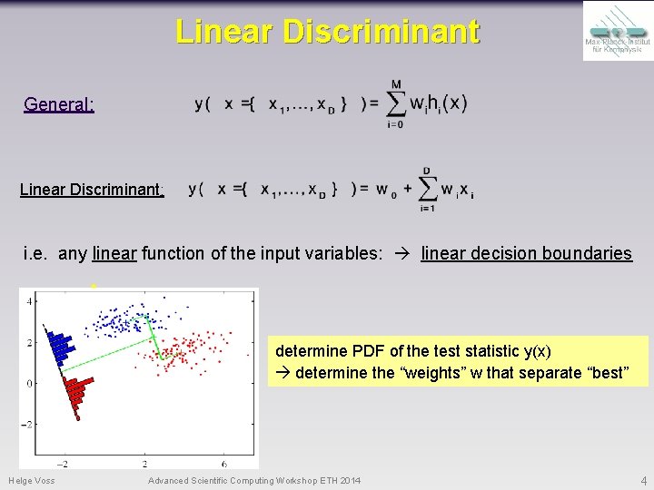
Linear Discriminant General: Linear Discriminant: i. e. any linear function of the input variables: linear decision boundaries x 2 H 1 determine PDF of the test statistic y(x) determine the “weights” w that separate “best” H 0 x 1 Helge Voss Advanced Scientific Computing Workshop ETH 2014 4

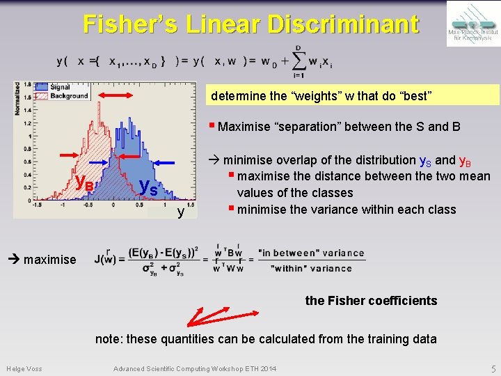
Fisher’s Linear Discriminant determine the “weights” w that do “best” § Maximise “separation” between the S and B y. S y minimise overlap of the distribution y. S and y. B § maximise the distance between the two mean values of the classes § minimise the variance within each class maximise the Fisher coefficients note: these quantities can be calculated from the training data Helge Voss Advanced Scientific Computing Workshop ETH 2014 5

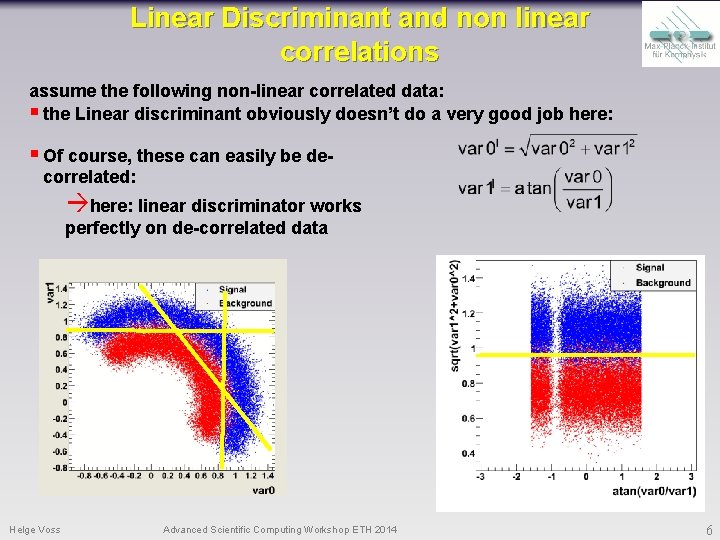
Linear Discriminant and non linear correlations assume the following non-linear correlated data: § the Linear discriminant obviously doesn’t do a very good job here: § Of course, these can easily be decorrelated: here: linear discriminator works perfectly on de-correlated data Helge Voss Advanced Scientific Computing Workshop ETH 2014 6

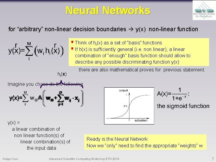
Neural Networks for “arbitrary” non-linear decision boundaries y(x) non-linear function § Think of hi(x) as a set of “basis” functions § If h(x) is sufficiently general (i. e. non linear), a linear combination of “enough” basis function should allow to describe any possible discriminating function y(x) hi(x) there also mathematical proves for previous statement. Imagine you chose do the following: y(x) = a linear combination of non linear function(s) of linear combination(s) of the input data Helge Voss Ready is the Neural Network Now we “only” need to find the appropriate “weights” w Advanced Scientific Computing Workshop ETH 2014 7

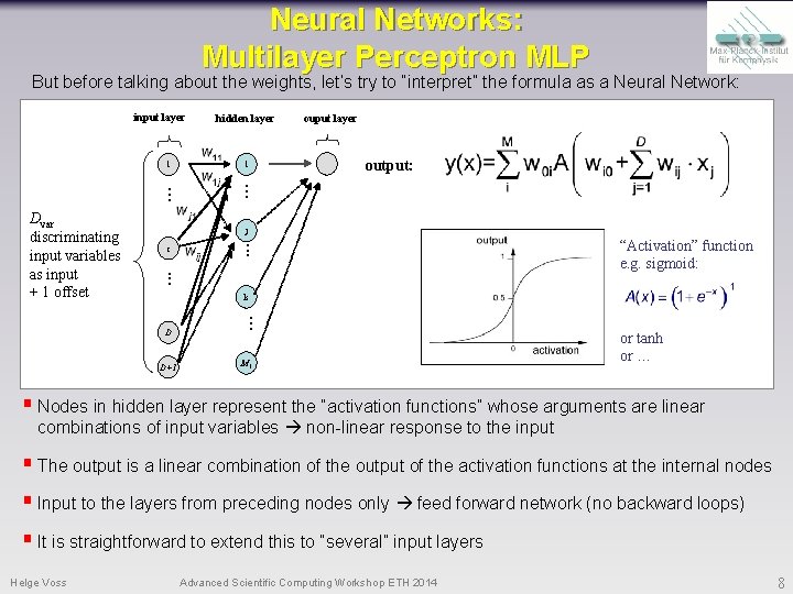
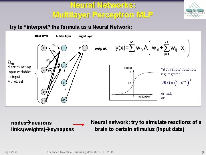
Neural Networks: Multilayer Perceptron MLP But before talking about the weights, let’s try to “interpret” the formula as a Neural Network: input layer 1 . . . Dvar discriminating input variables as input + 1 offset hidden layer 1 . . . ouput layer output: j i . . . k D D+1 . . . M 1 “Activation” function e. g. sigmoid: or tanh or … § Nodes in hidden layer represent the “activation functions” whose arguments are linear combinations of input variables non-linear response to the input § The output is a linear combination of the output of the activation functions at the internal nodes § Input to the layers from preceding nodes only feed forward network (no backward loops) § It is straightforward to extend this to “several” input layers Helge Voss Advanced Scientific Computing Workshop ETH 2014 8

Neural Networks: Multilayer Perceptron MLP try to “interpret” the formula as a Neural Network: input layer 1 . . . Dvar discriminating input variables as input + 1 offset hidden layer 1 . . . output: j i . . . k D D+1 “Activation” function e. g. sigmoid: . . . or tanh or … M 1 nodes neurons links(weights) synapses Helge Voss ouput layer Neural network: try to simulate reactions of a brain to certain stimulus (input data) Advanced Scientific Computing Workshop ETH 2014 9

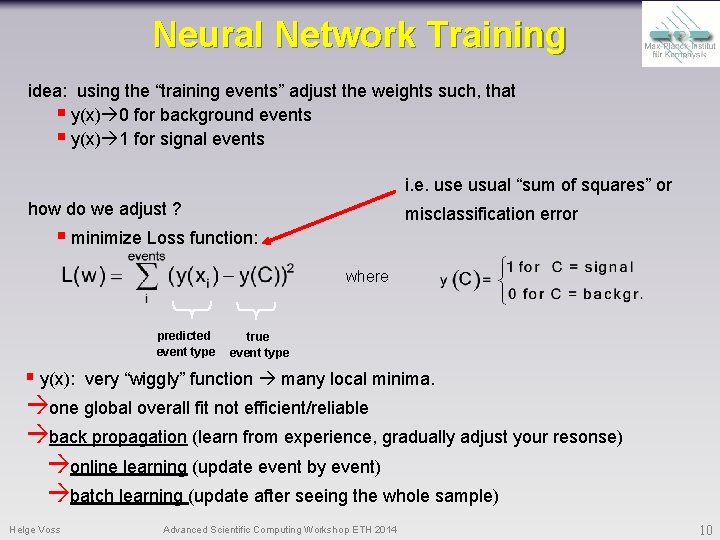
Neural Network Training idea: using the “training events” adjust the weights such, that § y(x) 0 for background events § y(x) 1 for signal events i. e. use usual “sum of squares” or how do we adjust ? misclassification error § minimize Loss function: where predicted event type true event type § y(x): very “wiggly” function many local minima. one global overall fit not efficient/reliable back propagation (learn from experience, gradually adjust your resonse) online learning (update event by event) batch learning (update after seeing the whole sample) Helge Voss Advanced Scientific Computing Workshop ETH 2014 10

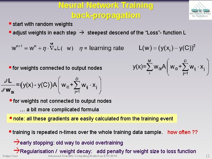
Neural Network Training back-propagation § start with random weights § adjust weights in each step steepest descend of the “Loss”- function L § for weights connected to output nodes § for weights not connected to output nodes … a bit more complicated formula § note: all these gradients are easily calculated from the training event § training is repeated n-times over the whole training data sample. how often ? ? early stopping: old way to avoid overtraining Regularisation / weight decay: add penalty for weight size to loss function Helge Voss Advanced Scientific Computing Workshop ETH 2014 11

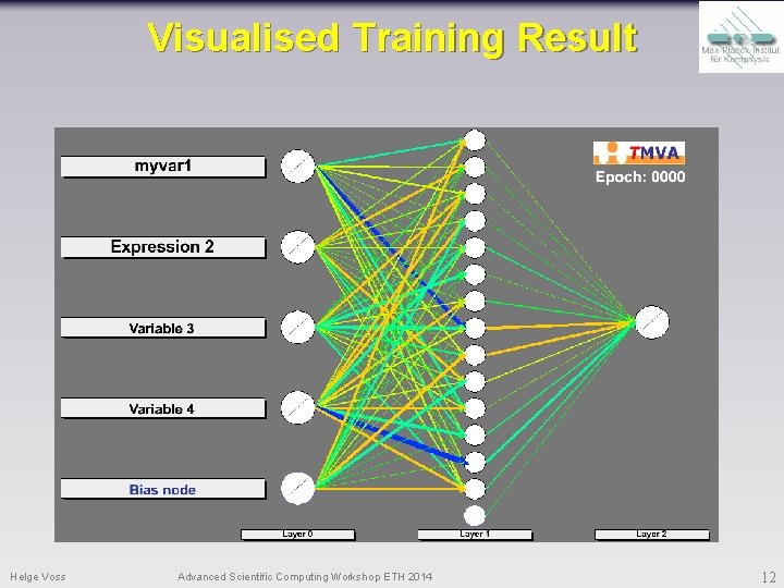
Visualised Training Result Helge Voss Advanced Scientific Computing Workshop ETH 2014 12

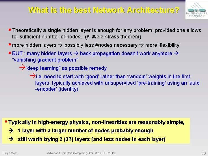
What is the best Network Architecture? § Theoretically a single hidden layer is enough for any problem, provided one allows for sufficient number of nodes. (K. Weierstrass theorem) § more hidden layers possibly less #nodes necessary more ‘flexibility’ § BUT : many hidden layers back propagation doesn’t work anymore “vanishing gradient problem” “deep learning” as possible remedy i. e. need to start with ‘good’ rather than ‘random’ weights in the first layers, typically achieved with unsupervised ‘pre-training’ using an ‘auto -encoder’ (identity) § Typically in high-energy physics, non-linearities are reasonably simple, 1 layer with a larger number of nodes probably enough still worth trying 2 (3? ) layers (and less nodes in each layer) Helge Voss Advanced Scientific Computing Workshop ETH 2014 13

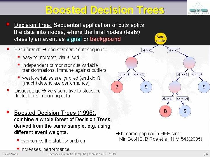
Boosted Decision Trees § Decision Tree: Sequential application of cuts splits the data into nodes, where the final nodes (leafs) classify an event as signal or background § Each branch one standard “cut” sequence § § easy to interpret, visualised § weak variables are ignored (and don’t (much) deteriorate performance) independent of monotonous variable transformations, immune against outliers § Disadvatage very sensitive to statistical fluctuations in training data § Boosted Decision Trees (1996): combine a whole forest of Decision Trees, derived from the sample, e. g. using different event weights. became popular in HEP since § overcomes the stability problem § increases performance Helge Voss Advanced Scientific Computing Workshop ETH 2014 Mini. Boo. NE, B. Roe et. a. , NIM 543(2005) 14

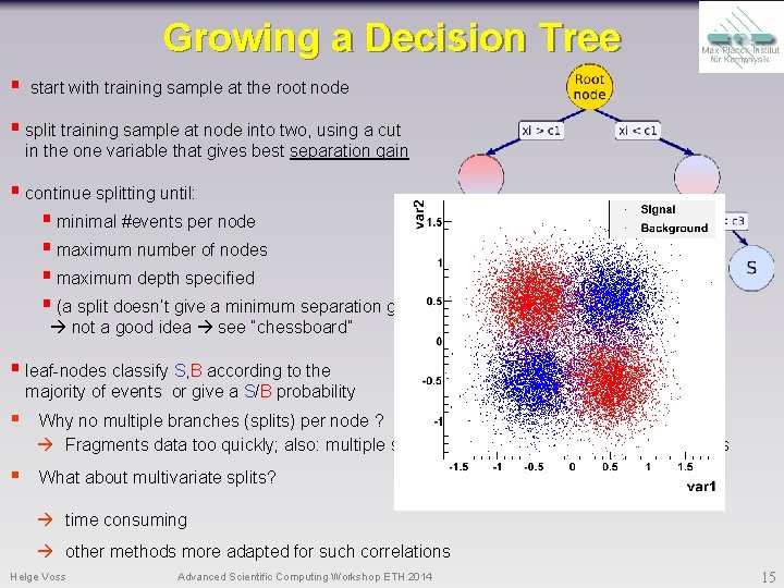
Growing a Decision Tree § start with training sample at the root node § split training sample at node into two, using a cut in the one variable that gives best separation gain § continue splitting until: § minimal #events per node § maximum number of nodes § maximum depth specified § (a split doesn’t give a minimum separation gain) not a good idea see “chessboard” § leaf-nodes classify S, B according to the majority of events or give a S/B probability § Why no multiple branches (splits) per node ? Fragments data too quickly; also: multiple splits per node = series of binary node splits § What about multivariate splits? time consuming other methods more adapted for such correlations Helge Voss Advanced Scientific Computing Workshop ETH 2014 15

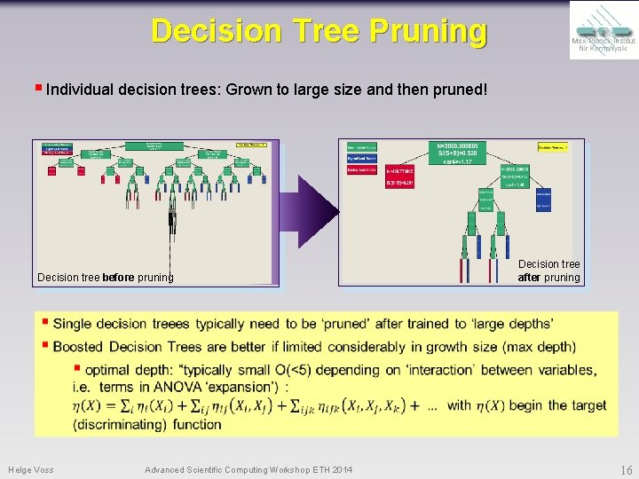
Decision Tree Pruning § Individual decision trees: Grown to large size and then pruned! Decision tree before pruning Decision tree after pruning Helge Voss Advanced Scientific Computing Workshop ETH 2014 16

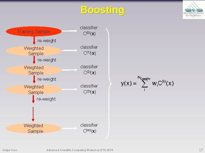
Boosting Training Sample classifier C(0)(x) re-weight Helge Voss Weighted Sample re-weight classifier C(1)(x) Weighted Sample re-weight classifier C(2)(x) Weighted Sample re-weight classifier C(3)(x) Weighted Sample classifier C(m)(x) Advanced Scientific Computing Workshop ETH 2014 17

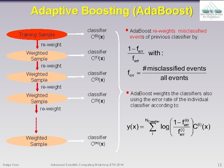
Adaptive Boosting (Ada. Boost) Training Sample classifier C(0)(x) § Ada. Boost re-weights misclassified events of previous classifier by: re-weight Helge Voss Weighted Sample re-weight classifier C(1)(x) Weighted Sample re-weight classifier C(2)(x) Weighted Sample re-weight classifier C(3)(x) Weighted Sample classifier C(m)(x) Advanced Scientific Computing Workshop ETH 2014 § Ada. Boost weights the classifiers also using the error rate of the individual classifier according to: 18

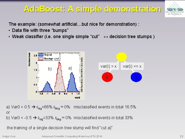
Ada. Boost: A simple demonstration The example: (somewhat artificial…but nice for demonstration) : • Data file with three “bumps” • Weak classifier (i. e. one single simple “cut” ↔ decision tree stumps ) b) a) var(i) > x B var(i) <= x S a) Var 0 > 0. 5 εsig=66% εbkg ≈ 0% misclassified events in total 16. 5% or b) Var 0 < -0. 5 εsig=33% εbkg ≈ 0% misclassified events in total 33% the training of a single decision tree stump will find “cut a)” Helge Voss Advanced Scientific Computing Workshop ETH 2014 19

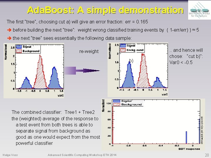
Ada. Boost: A simple demonstration The first “tree”, choosing cut a) will give an error fraction: err = 0. 165 before building the next “tree”: weight wrong classified training events by ( 1 -err/err) ) ≈ 5 the next “tree” sees essentially the following data sample: re-weight b) . . and hence will chose: “cut b)”: Var 0 < -0. 5 The combined classifier: Tree 1 + Tree 2 the (weighted) average of the response to a test event from both trees is able to separate signal from background as good as one would expect from the most powerful classifier Helge Voss Advanced Scientific Computing Workshop ETH 2014 20

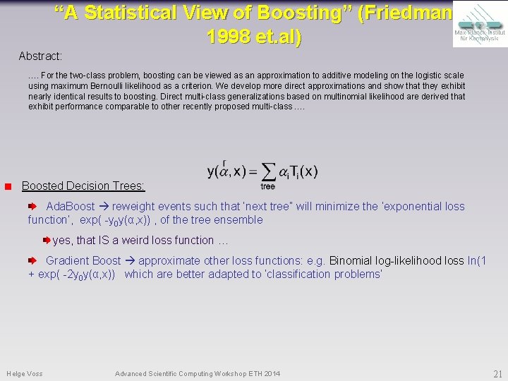
“A Statistical View of Boosting” (Friedman 1998 et. al) Abstract: …. For the two-class problem, boosting can be viewed as an approximation to additive modeling on the logistic scale using maximum Bernoulli likelihood as a criterion. We develop more direct approximations and show that they exhibit nearly identical results to boosting. Direct multi-class generalizations based on multinomial likelihood are derived that exhibit performance comparable to other recently proposed multi-class …. Boosted Decision Trees: Ada. Boost reweight events such that ‘next tree” will minimize the ‘exponential loss function’, exp( -y 0 y(α, x)) , of the tree ensemble yes, that IS a weird loss function … Gradient Boost approximate other loss functions: e. g. Binomial log-likelihood loss ln(1 + exp( -2 y 0 y(α, x)) which are better adapted to ‘classification problems’ Helge Voss Advanced Scientific Computing Workshop ETH 2014 21

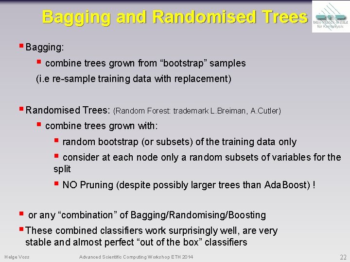
Bagging and Randomised Trees § Bagging: § combine trees grown from “bootstrap” samples (i. e re-sample training data with replacement) § Randomised Trees: (Random Forest: trademark L. Breiman, A. Cutler) § combine trees grown with: § random bootstrap (or subsets) of the training data only § consider at each node only a random subsets of variables for the split § NO Pruning (despite possibly larger trees than Ada. Boost) ! § or any “combination” of Bagging/Randomising/Boosting § These combined classifiers work surprisingly well, are very stable and almost perfect “out of the box” classifiers Helge Voss Advanced Scientific Computing Workshop ETH 2014 22

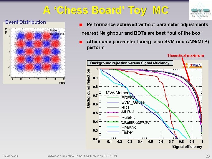
A ‘Chess Board’ Toy MC Event Distribution Performance achieved without parameter adjustments: nearest Neighbour and BDTs are best “out of the box” After some parameter tuning, also SVM und ANN(MLP) perform Theoretical maximum Helge Voss Advanced Scientific Computing Workshop ETH 2014 23

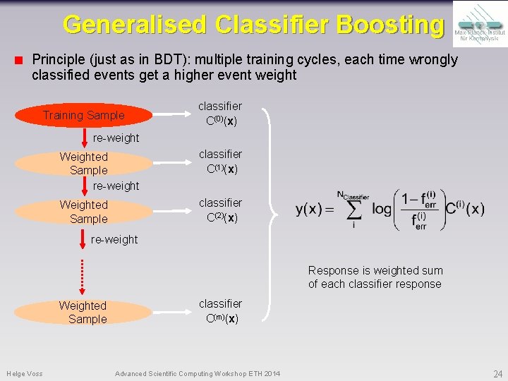
Generalised Classifier Boosting Principle (just as in BDT): multiple training cycles, each time wrongly classified events get a higher event weight Training Sample classifier C(0)(x) re-weight Weighted Sample re-weight classifier C(1)(x) Weighted Sample classifier C(2)(x) re-weight Response is weighted sum of each classifier response Weighted Sample Helge Voss classifier C(m)(x) Advanced Scientific Computing Workshop ETH 2014 24

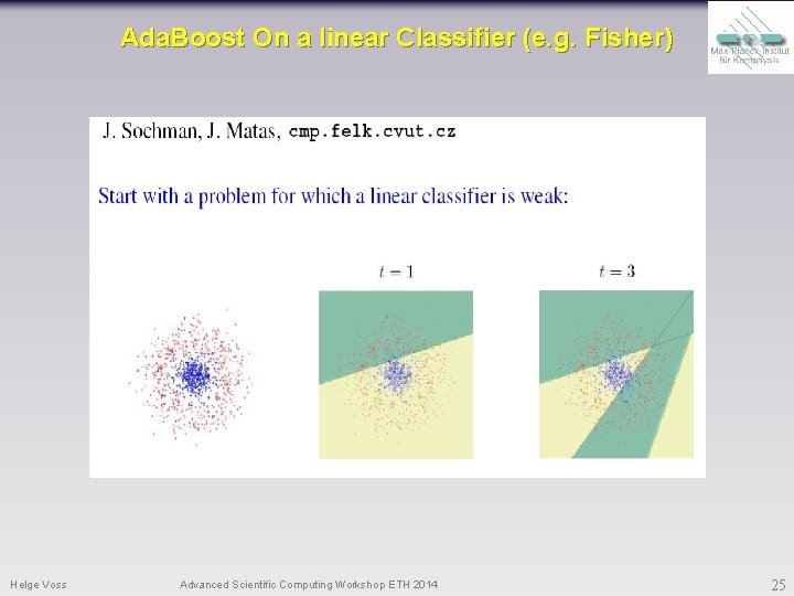
Ada. Boost On a linear Classifier (e. g. Fisher) Helge Voss Advanced Scientific Computing Workshop ETH 2014 25

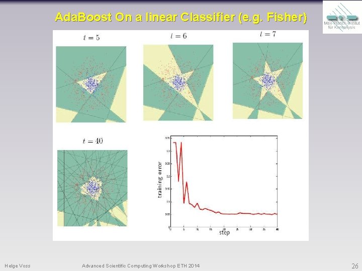
Ada. Boost On a linear Classifier (e. g. Fisher) Helge Voss Advanced Scientific Computing Workshop ETH 2014 26

Support Vector Machines § Neural Networks are complicated by finding the proper optimum “weights” for best separation power by “wiggly” functional behaviour of the piecewise defined separating hyperplane § KNN (multidimensional likelihood) suffers disadvantage that calculating the MVA-output of each test event involves evaluation of ALL training events § If Boosted Decision Trees in theory are always weaker than a perfect Neural Network Helge Voss Advanced Scientific Computing Workshop ETH 2014 27

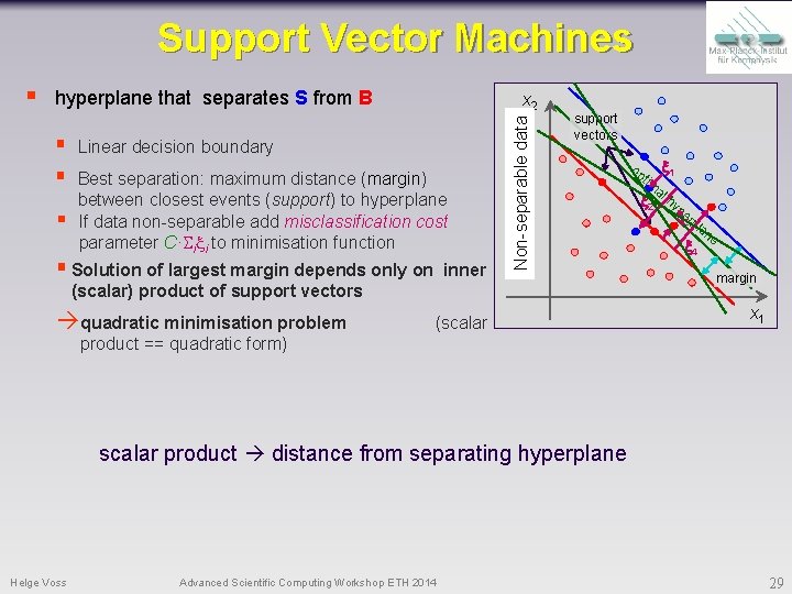
Support Vector Machine § There are methods to create linear decision boundaries using only measures of distances (= inner (scalar) products) § leads to quadratic optimisation problem § The decision boundary in the end is defined only by training events that are closest to the boundary § suitable variable transformations into a higher dimensional space may allow separation with linear decision boundaries non linear problems § Support Vector Machine Helge Voss Advanced Scientific Computing Workshop ETH 2014 28

Support Vector Machines hyperplane that separates S from B § § § x 2 Linear decision boundary Best separation: maximum distance (margin) between closest events (support) to hyperplane If data non-separable add misclassification cost parameter C· i i to minimisation function § Solution of largest margin depends only on inner Separable data Non-separable § support vectors (scalar) product of support vectors quadratic minimisation problem (scalar op tim 1 a 2 l hyp e 3 rp la 4 ne margin x 1 product == quadratic form) scalar product distance from separating hyperplane Helge Voss Advanced Scientific Computing Workshop ETH 2014 29

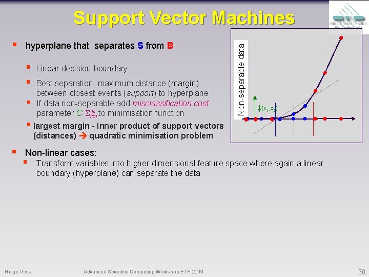
§ hyperplane that separates S from B § § § Linear decision boundary Best separation: maximum distance (margin) between closest events (support) to hyperplane If data non-separable add misclassification cost parameter C· i i to minimisation function Separable data Non-separable Support Vector Machines (x 1, x 2) § largest margin - inner product of support vectors (distances) quadratic minimisation problem § Non-linear cases: § Helge Voss Transform variables into higher dimensional feature space where again a linear boundary (hyperplane) can separate the data Advanced Scientific Computing Workshop ETH 2014 30

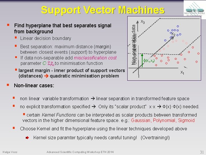
Support Vector Machines Find hyperplane that best separates signal from background § § § Linear decision boundary Best separation: maximum distance (margin) between closest events (support) to hyperplane If data non-separable add misclassification cost parameter C· i i to minimisation function Non-separable Separable data § x 3 xx 22 (x 1, x 2) § largest margin - inner product of support vectors (distances) quadratic minimisation problem § xx 11 x 1 Non-linear cases: § § non linear variable transformation linear separation in transformed feature space no explicit transformation specified Only its “scalar product” x·x Ф(x)·Ф(x) needed. § certain Kernel Functions can be interpreted as scalar products between transformed vectors in the higher dimensional feature space. e. g. : Gaussian, Polynomial, Sigmoid § Choose Kernel and fit the hyperplane using the linear techniques developed above Kernel size paramter typically needs careful tuning! (Overtraining!) Helge Voss Advanced Scientific Computing Workshop ETH 2014 31

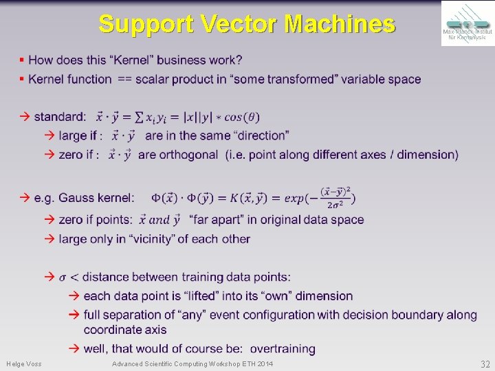
Support Vector Machines Helge Voss Advanced Scientific Computing Workshop ETH 2014 32

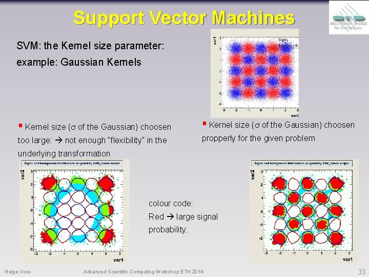
Support Vector Machines SVM: the Kernel size parameter: example: Gaussian Kernels § Kernel size (s of the Gaussian) choosen too large: not enough “flexibility” in the propperly for the given problem underlying transformation colour code: Red large signal probability: Helge Voss Advanced Scientific Computing Workshop ETH 2014 33