Multivariate Methods of data analysis Advanced Scientific Computing

Multivariate Methods of data analysis Advanced Scientific Computing Workshop ETH 2014 Helge Voss MAX-PLANCK-INSTITUT FÜR KERNPHYSIK IN HEIDELBERG Helge Voss Advanced Scientific Computing Workshop ETH 2014 1

Overview § Multivariate classification/regression algorithms (MVA) § what they are § how they work § Overview over some classifiers § Multidimensional Likelihood (k. NN : k-Nearest Neighbour) § Projective Likelihood (naïve Bayes) § Linear Classifier § Non linear Classifiers § Neural Networks § Boosted Decision Trees § Support Vector Machines § General comments about: § Overtraining Helge Voss § Systematic errors Advanced Scientific Computing Workshop ETH 2014 2

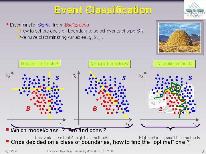
Event Classification § Discriminate Signal from Background § how to set the decision boundary to select events of type S ? § we have discriminating variables x 1, x 2, … Rectangular cuts? x 2 A linear boundary? x 2 S B x 1 A nonlinear one? S B x 1 § Which model/class ? Pro and cons ? Low variance (stable), high bias methods High variance, small bias methods § Once decided on a class of boundaries, how to find the “optimal” one ? Helge Voss Advanced Scientific Computing Workshop ETH 2014 3

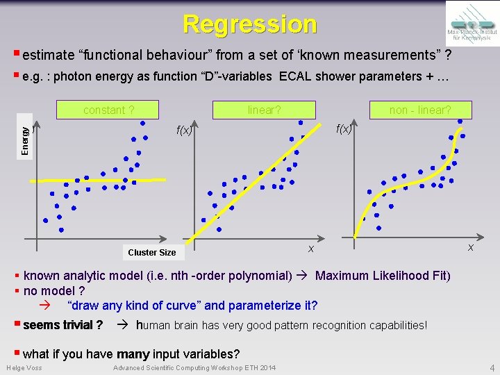
Regression § estimate “functional behaviour” from a set of ‘known measurements” ? § e. g. : photon energy as function “D”-variables constant ? ECAL shower parameters + … linear? non - linear? f(x) Energy f(x) x Size Cluster x x § known analytic model (i. e. nth -order polynomial) Maximum Likelihood Fit) § no model ? “draw any kind of curve” and parameterize it? § seems trivial ? human brain has very good pattern recognition capabilities! § what if you have many input variables? Helge Voss Advanced Scientific Computing Workshop ETH 2014 4

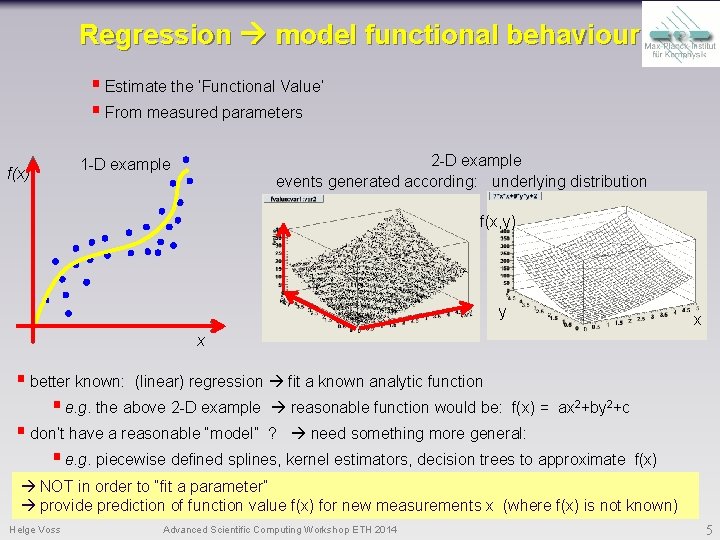
Regression model functional behaviour § Estimate the ‘Functional Value’ § From measured parameters f(x) 2 -D example events generated according: underlying distribution 1 -D example f(x, y) y x x § better known: (linear) regression fit a known analytic function § e. g. the above 2 -D example reasonable function would be: f(x) = ax 2+by 2+c § don’t have a reasonable “model” ? need something more general: § e. g. piecewise defined splines, kernel estimators, decision trees to approximate f(x) NOT in order to “fit a parameter” provide prediction of function value f(x) for new measurements x (where f(x) is not known) Helge Voss Advanced Scientific Computing Workshop ETH 2014 5

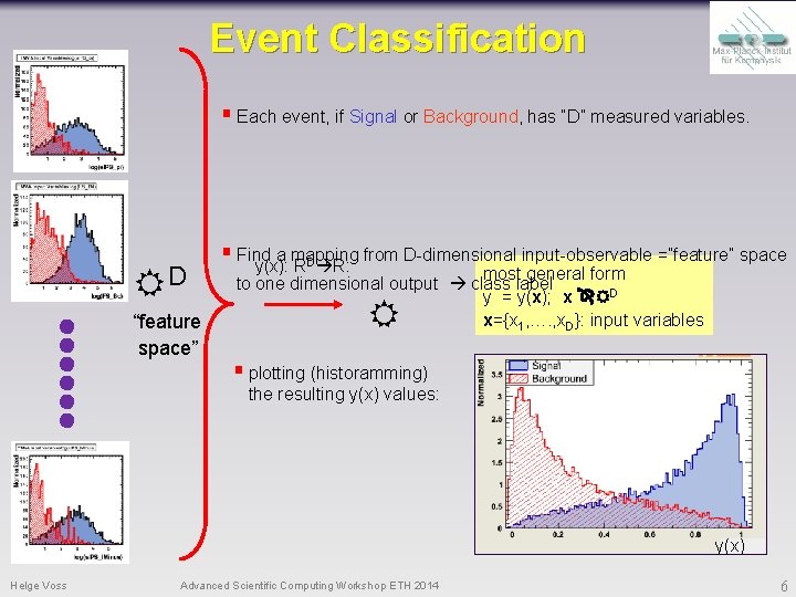
Event Classification § Each event, if Signal or Background, has “D” measured variables. D “feature space” § Find a mapping from D-dimensional input-observable =”feature” space y(x): RD R: most general form to one dimensional output class label y = y(x); x D x={x 1, …. , x. D}: input variables § plotting (historamming) the resulting y(x) values: y(x) Helge Voss Advanced Scientific Computing Workshop ETH 2014 6

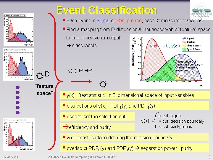
Event Classification § Each event, if Signal or Background, has “D” measured variables. § Find a mapping from D-dimensional input/observable/”feature” space to one dimensional output y(B) 0, y(S) 1 class labels D “feature space” y(x): Rn R: § y(x): “test statistic” in D-dimensional space of input variables § distributions of y(x): PDFS(y) and PDFB(y) § used to set the selection cut! efficiency and purity y(x): > cut: signal = cut: decision boundary < cut: background § y(x)=const: surface defining the decision boundary. § overlap of PDFS(y) and PDFB(y) separation power , purity Helge Voss Advanced Scientific Computing Workshop ETH 2014 7

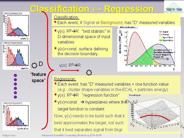
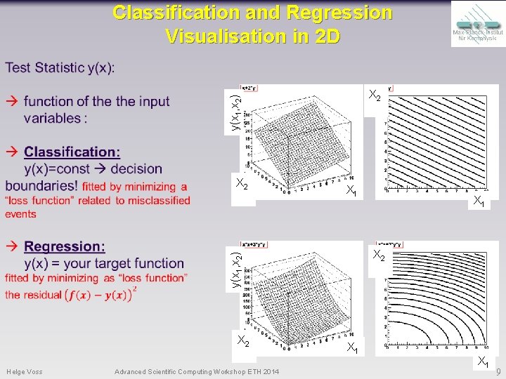
Classification ↔ Regression Classification: § Each event, if Signal or Background, has “D” measured variables. § y(x): RD R: “test statistic” in D-dimensional space of input variables § y(x)=const: surface defining the decision boundary. D “feature space” y(x): RD R: Regression: § Each event has “D” measured variables + one function value (e. g. cluster shape variables in the ECAL + particles energy) § y(x): RD R “regression function” § y(x)=const hyperplanes where thef(x 1, x 2) target function is constant Now, y(x) needs to be build such that it best approximates the target, not such that it best separates signal from bkgr. Helge Voss Advanced Scientific Computing Workshop ETH 2014 X 2 X 1 8

Classification and Regression Visualisation in 2 D y(x 1, x 2) X 2 X 1 X 2 Helge Voss Advanced Scientific Computing Workshop ETH 2014 X 1 X 2 y(x 1, x 2) X 2 X 1 9

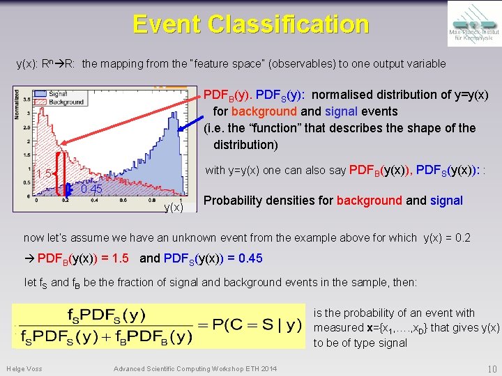
Event Classification y(x): Rn R: the mapping from the “feature space” (observables) to one output variable PDFB(y). PDFS(y): normalised distribution of y=y(x) for background and signal events (i. e. the “function” that describes the shape of the distribution) with y=y(x) one can also say PDFB(y(x)), PDFS(y(x)): : 1. 5 0. 45 y(x) Probability densities for background and signal now let’s assume we have an unknown event from the example above for which y(x) = 0. 2 PDFB(y(x)) = 1. 5 and PDFS(y(x)) = 0. 45 let f. S and f. B be the fraction of signal and background events in the sample, then: is the probability of an event with measured x={x 1, …. , x. D} that gives y(x) to be of type signal Helge Voss Advanced Scientific Computing Workshop ETH 2014 10

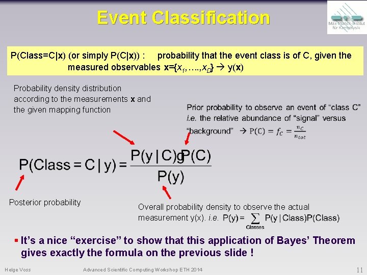
Event Classification P(Class=C|x) (or simply P(C|x)) : probability that the event class is of C, given the measured observables x={x 1, …. , x. D} y(x) Probability density distribution according to the measurements x and the given mapping function Posterior probability Overall probability density to observe the actual measurement y(x). i. e. § It’s a nice “exercise” to show that this application of Bayes’ Theorem gives exactly the formula on the previous slide ! Helge Voss Advanced Scientific Computing Workshop ETH 2014 11

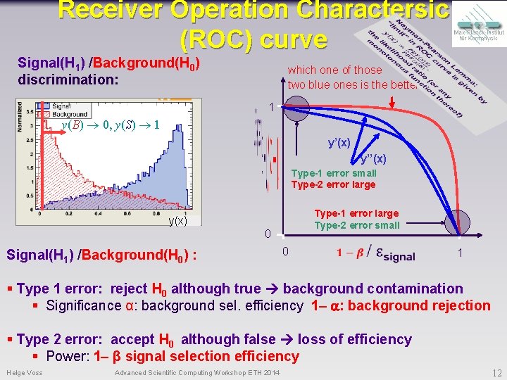
Receiver Operation Charactersic (ROC) curve Signal(H 1) /Background(H 0) discrimination: which one of those two blue ones is the better? ? 1 y(B) 0, y(S) 1 y’(x) y’’(x) Type-1 error small Type-2 error large Type-1 error large Type-2 error small y(x) 0 Signal(H 1) /Background(H 0) : 0 1 § Type 1 error: reject H 0 although true background contamination § Significance α: background sel. efficiency 1 - a: background rejection § Type 2 error: accept H 0 although false loss of efficiency § Power: 1 - β signal selection efficiency Helge Voss Advanced Scientific Computing Workshop ETH 2014 12

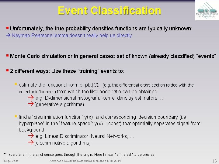
Event Classification § Unfortunately, the true probability densities functions are typically unknown: Neyman-Pearsons lemma doesn’t really help us directly § Monte Carlo simulation or in general cases: set of known (already classified) “events” § 2 different ways: Use these “training” events to: § estimate the functional form of p(x|C): (e. g. the differential cross section folded with the detector influences) from which the likelihood ratio can be obtained e. g. D-dimensional histogram, Kernel densitiy estimators, … (generative algorithms) § find a “discrimination function” y(x) and corresponding decision boundary (i. e. hyperplane* in the “feature space”: y(x) = const) that optimially separates signal from background e. g. Linear Discriminator, Neural Networks, … (discriminative algorithms) * hyperplane in the strict sense goes through the origin. Here I mean “affine set” to be precise Helge Voss Advanced Scientific Computing Workshop ETH 2014 13

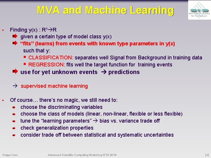
MVA and Machine Learning § Finding y(x) : Rn R given a certain type of model class y(x) “fits” (learns) from events with known type parameters in y(x) such that y: § CLASSIFICATION: separates well Signal from Background in training data § REGRESSION: fits well the target function for training events use for yet unknown events predictions supervised machine learning § Of course… there’s no magic, we still need to: choose the discriminating variables choose the class of models (linear, non-linear, flexible or less flexible) tune the “learning parameters” bias vs. variance trade off check generalization properties consider trade off between statistical and systematic uncertainties Helge Voss Advanced Scientific Computing Workshop ETH 2014 14

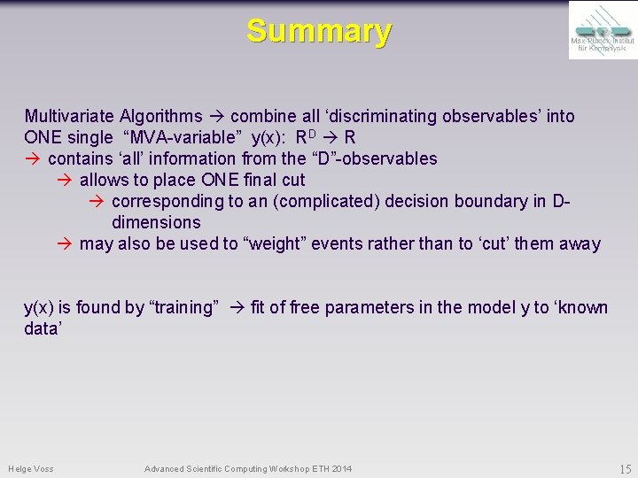
Summary Multivariate Algorithms combine all ‘discriminating observables’ into ONE single “MVA-variable” y(x): RD R contains ‘all’ information from the “D”-observables allows to place ONE final cut corresponding to an (complicated) decision boundary in Ddimensions may also be used to “weight” events rather than to ‘cut’ them away y(x) is found by “training” fit of free parameters in the model y to ‘known data’ Helge Voss Advanced Scientific Computing Workshop ETH 2014 15