Multivariate Cointegartion The Johansen Maximum Likelihood Procedure Granger

Multivariate Cointegartion The Johansen Maximum Likelihood Procedure

Granger Causality Tests Continued • According to Granger, causality can be further subdivided into long-run and short-run causality. • This requires the use of error correction models or VECMs, depending on the approach for determining causality. • Long-run causality is determined by the error correction term, whereby if it is significant, then it indicates evidence of long run causality from the explanatory variable to the dependent variable. • Short-run causality is determined as before, with a test on the joint significance of the lagged explanatory variables, using an F-test or Wald test.

Long-run Causality • Before the ECM can be formed, there first has to be evidence of cointegration, given that cointegration implies a significant error correction term, cointegration can be viewed as an indirect test of long-run causality. • It is possible to have evidence of long-run causality, but not short-run causality and vice versa. • In multivariate causality tests, the testing of long-run causality between two variables is more problematic, as it is impossible to tell which explanatory variable is causing the causality through the error correction term.

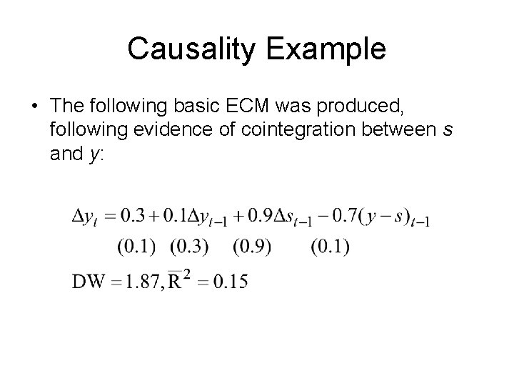
Causality Example • The following basic ECM was produced, following evidence of cointegration between s and y:

Causality Example • In the previous example, there is long-run causality between s to y, as the error correction term is significant (t-ratio of 7). • There is no evidence of short-run causality as the lagged differenced explanatory variable is insignificant (t-ratio of 1, an Ftest would also include insignificance).

Introduction • Describe the Johansen Approach to cointegration • Assess the Trace and Maximal Eigenvalue test statistics • Illustrate the use of the Johansen approach, including the long and short run effects. • Critically appraise the Johansen approach to cointegration

Multivariate Approach to Cointegration • Using the Johansen Maximum Likelihood (ML) procedure, it is possible to obtain more then a single cointegrating relationship. • If there is evidence of more than one cointegrating relationship, which one should be used? • There are two separate tests for cointegration, which can give different results. • Given that this is a maximum likelihood based test (Engle -Granger is OLS based), it requires a large sample. • The multivariate test is based on a VAR, not a single OLS estimation.

The Johansen ML Procedure • This is based on a VAR approach to cointegration • All the variables are assumed to be endogenous (although it is possible to include exogenous variables) • The test relies on the relationship between the rank of a matrix and its eigenvalues or characteristic roots. You do not need to understand the mechanics of this approach, just how to use it and how to interpret the results

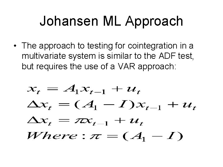
Johansen ML Approach • The approach to testing for cointegration in a multivariate system is similar to the ADF test, but requires the use of a VAR approach:

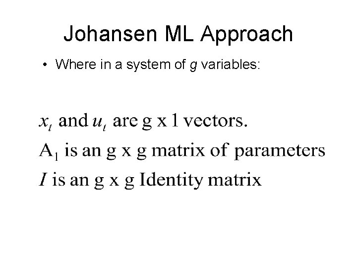
Johansen ML Approach • Where in a system of g variables:

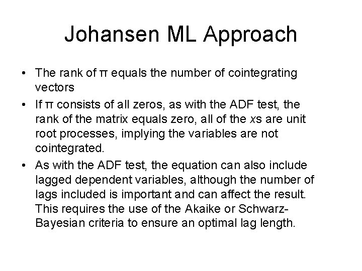
Johansen ML Approach • The rank of π equals the number of cointegrating vectors • If π consists of all zeros, as with the ADF test, the rank of the matrix equals zero, all of the xs are unit root processes, implying the variables are not cointegrated. • As with the ADF test, the equation can also include lagged dependent variables, although the number of lags included is important and can affect the result. This requires the use of the Akaike or Schwarz. Bayesian criteria to ensure an optimal lag length.

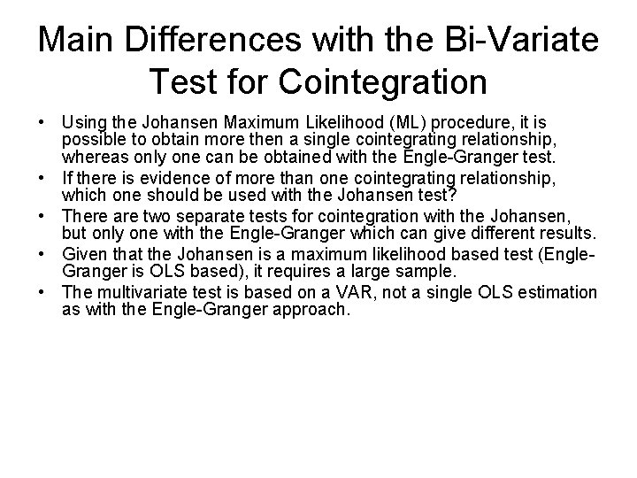
Main Differences with the Bi-Variate Test for Cointegration • Using the Johansen Maximum Likelihood (ML) procedure, it is possible to obtain more then a single cointegrating relationship, whereas only one can be obtained with the Engle-Granger test. • If there is evidence of more than one cointegrating relationship, which one should be used with the Johansen test? • There are two separate tests for cointegration with the Johansen, but only one with the Engle-Granger which can give different results. • Given that the Johansen is a maximum likelihood based test (Engle. Granger is OLS based), it requires a large sample. • The multivariate test is based on a VAR, not a single OLS estimation as with the Engle-Granger approach.

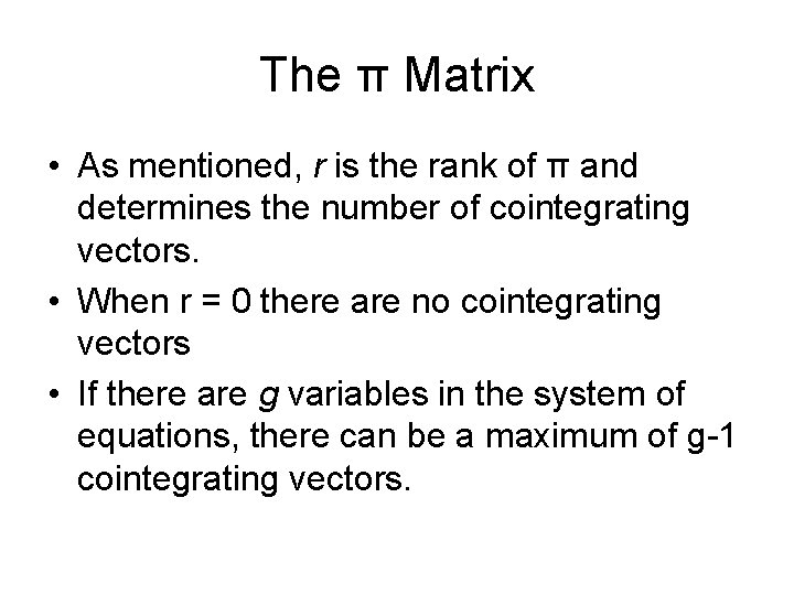
The π Matrix • As mentioned, r is the rank of π and determines the number of cointegrating vectors. • When r = 0 there are no cointegrating vectors • If there are g variables in the system of equations, there can be a maximum of g-1 cointegrating vectors.

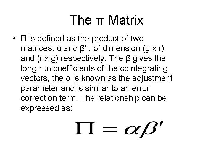
The π Matrix • Π is defined as the product of two matrices: α and β’ , of dimension (g x r) and (r x g) respectively. The β gives the long-run coefficients of the cointegrating vectors, the α is known as the adjustment parameter and is similar to an error correction term. The relationship can be expressed as:

Test Statistics • There are two test statistics produced by the Johansen ML procedure. • There are the Trace test and maximal Eigenvalue test. • Both can be used to determine the number of cointegrating vectors present, although they don’t always indicate the same number of cointegrating vectors.

Differences Between the Two Test Statistics • The Trace test is a joint test, the null hypothesis is that the number of cointegrating vectors is less than or equal to r, against a general alternative hypothesis that there are more then r. • The Maximal Eigenvalue test conducts separate tests on each eigenvalue. The null hypothesis is that there are r cointegrating vectors present against the alternative that there are (r + 1) present. • The distribution of both test statistics is nonstandard.

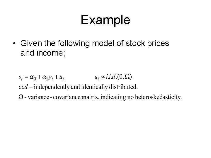
Example • Given the following model of stock prices and income;

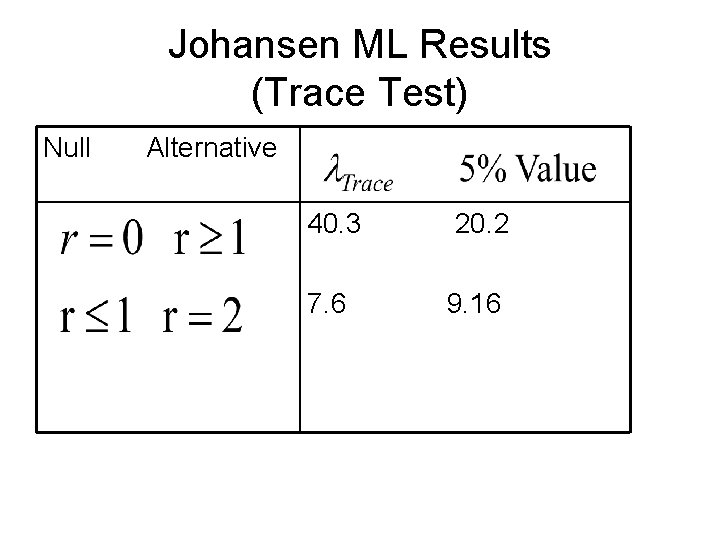
Johansen ML Results (Trace Test) Null Alternative 40. 3 20. 2 7. 6 9. 16

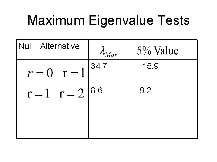
Maximum Eigenvalue Tests Null Alternative 34. 7 15. 9 8. 6 9. 2

Interpretation of Results • Given that for both tests, the test statistic exceeds its critical value (5%) when the null is r = 0, we can conclude that at least one cointegrating vector is present. • For more than one cointegrating vector, the test statistic is less than the critical value so we conclude only a single cointegrating vector is present.

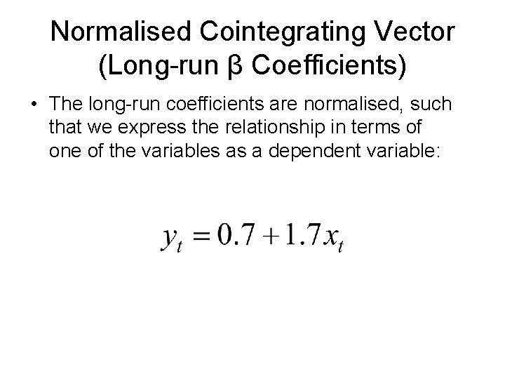
Normalised Cointegrating Vector (Long-run β Coefficients) • The long-run coefficients are normalised, such that we express the relationship in terms of one of the variables as a dependent variable:

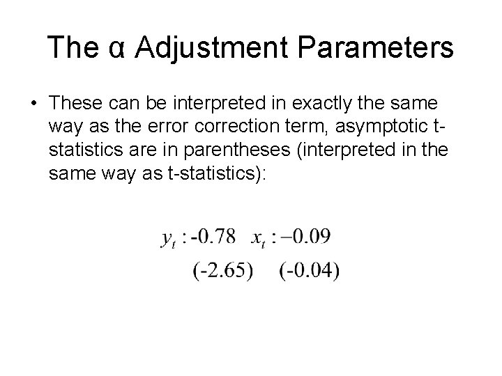
The α Adjustment Parameters • These can be interpreted in exactly the same way as the error correction term, asymptotic tstatistics are in parentheses (interpreted in the same way as t-statistics):

Tests of Specific Restrictions • The Johansen ML approach, unlike the bivariate approach can be used to apply certain restrictions to the long-run β coefficients. • This can involve testing if they are significantly different to zero or not, or equal to one.

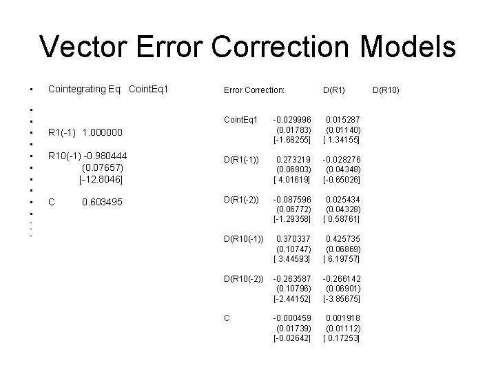
Multivariate Cointegration and VECMs • Vector Error Correction Models (VECM) are the basic VAR, with an error correction term incorporated into the model and as with bivariate cointegration, multivariate cointegration implies an appropriate VECM can be formed. • The reason for the error correction term is the same as with the standard error correction model, it measures any movement away from the long-run equilibrium. • These are often used as part of a multivariate test for cointegration, such as the Johansen ML test, having found evidence of cointegration of some I(1) variables, we can then assess the short run and potential Granger causality with a VECM.

Vector Error Correction Models • • • • Cointegrating Eq: Coint. Eq 1 Error Correction: D(R 1) Coint. Eq 1 -0. 029996 (0. 01783) [-1. 68255] 0. 015287 (0. 01140) [ 1. 34155] D(R 1(-1)) 0. 273219 (0. 06803) [ 4. 01619] -0. 028276 (0. 04348) [-0. 65026] D(R 1(-2)) -0. 087596 (0. 06772) [-1. 29358] 0. 025434 (0. 04328) [ 0. 58761] D(R 10(-1)) 0. 370337 (0. 10747) [ 3. 44593] 0. 425735 (0. 06869) [ 6. 19757] D(R 10(-2)) -0. 263587 (0. 10796) [-2. 44152] -0. 266142 (0. 06901) [-3. 85675] C -0. 000459 (0. 01739) [-0. 02642] 0. 001918 (0. 01112) [ 0. 17253] R 1(-1) 1. 000000 R 10(-1) -0. 980444 (0. 07657) [-12. 8046] C 0. 603495 D(R 10)

Criticisms of the Johansen Approach • The result can be sensitive to the number of lags included in the test and the presence of autocorrelation • If there are more than two cointegrating vectors present, how do we find the most appropriate vector for the subsequent tests. • If the two test statistics differ, which one gives the correct result? • This is a large sample test. • The Wickens critique suggests we often find evidence of cointegration when none exists.

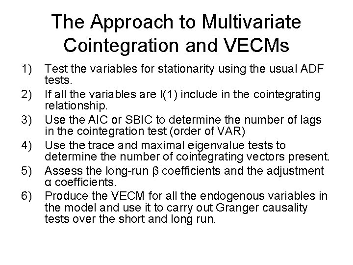
The Approach to Multivariate Cointegration and VECMs 1) 2) 3) 4) 5) 6) Test the variables for stationarity using the usual ADF tests. If all the variables are I(1) include in the cointegrating relationship. Use the AIC or SBIC to determine the number of lags in the cointegration test (order of VAR) Use the trace and maximal eigenvalue tests to determine the number of cointegrating vectors present. Assess the long-run β coefficients and the adjustment α coefficients. Produce the VECM for all the endogenous variables in the model and use it to carry out Granger causality tests over the short and long run.

Conclusion • When there are more than two variables, we need to use the Johansen ML approach to test for cointegration • There are two statistics to take into account; the trace and maximum eigenvalue. • Depending on how many cointegrating vectors are present, we can then test for the short-run using a vector error correction model.