Multivariate analysis in community ecology Gerry Quinn Deakin

Multivariate analysis in community ecology Gerry Quinn Deakin University

Data sets in community ecology • Multivariate abundance data • Sampling or experimental units – plots, cores, panels, quadrats …… – usually in hierarchical spatial or temporal structure • Abundances recorded for multiple taxa in each unit – simple counts, densities, % cover, presence-absence …… • Environmental variables recorded in each unit – p. H, salinity, temperature, nutrients, sediment load, elevation …. .

Typical aims • Examine spatial and temporal patterns in species composition – assemblage/community “structure”, more than simply biodiversity (e. g. taxon richness/diversity) – test formal hypotheses about spatial and temporal differences in composition • Relate patterns to unit (or higher) level environmental predictors – typical linear model type question • Determine which taxa are most important in “driving” the patterns – which taxa most typify differences across spatial and temporal hierarchies

Why multivariate? • Individual taxa of main interest – concern over multiple univariate hypothesis testing (Type 1 error rates) – referees and editors won’t accept paper with 50 -100 ANOVAs • Community (assemblage) structure interest – recognition of limitations of univariate biodiversity (richness, diversity, evenness) measures – hypotheses about community/assemblage composition • Most multivariate analyses in community ecology also incorporate univariate (individual taxa or environmental predictors) models

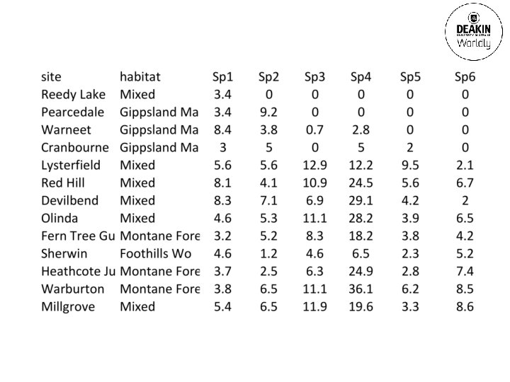
Forest bird communities • Does bird community composition vary between forest types? – 5 types (box-ironbark, river redgum, Gippsland manna gum etc. ) plus mixed • Maximum bird abundance (across 4 seasons) beechworthonline. com. au – 102 species across 37 sites • Mac Nally (1989) Swift parrot - Wikipedia

Estuary nematode communities • Does nematode community composition vary between sites and with environmental variables? • Nematode abundance (6 seasonal “replicates) – 182 species across 19 “sites” • Environmental variables Exe estuary - Wikipedia – 6 (sediment particle size, % organic matter etc. ) at each site • Clarke & Warwick (1993) Marine nematodes http: //www. ipm. iastate. edu

Site Sp 1 1 2 3 4 5 6 7 8 9 10 11 12 13 14 15 16 17 18 19 Sp 2 90 54 47 52 0 5 8 3 51 0 0 0 0 1 Sp 3 187 158 117 27 0 0 14 18 2 0 0 0 0 0 Sp 4 90 66 28 6 0 0 145 35 206 0 0 0 0 0 Sp 5 23 51 97 72 0 0 0 0 Sp 6 123 22 9 1 0 0 0 2 0 0 0 0 Sp 7 28 10 26 3 0 0 4 17 1 0 0 0 0 0 etc. 5 etc. 3 etc. 1 etc. 0 etc. 120 etc. 94 etc. 76 etc. 0 etc. Part WTab H 2 S Shore % size depth height organ Salinity 0. 06 0 2. 167 4 6. 43 24. 833 0. 06 0 3. 183 3 7. 06 22. 833 0. 06 0 1. 817 2 7. 99 17. 833 0. 06 0 2. 02 1 7. 15 16. 2 1. 275 20 20 5 0. 24 10 0. 562 3. 417 2. 95 4 0. 37 76. 6 0. 06 0 2. 167 3 1. 98 76 0. 177 0 2. 683 2 2. 22 81. 2 0. 06 0 2. 66 1 5. 88 71. 2 0. 451 20 20 5 0. 09 10 0. 205 4. 417 7. 25 4 0. 39 88 0. 528 20 20 3 0. 09 88 0. 598 20 20 2 0. 06 88 0. 769 0 20 1 0. 09 88. 5 0. 468 14. 917 20 5 0. 06 89 0. 837 6. 333 20 4 0. 04 90. 875 0. 797 6. 75 20 3 0. 06 91. 667 1. 141 3. 667 20 2 0. 07 89. 4 0. 223 0 20 1 0. 09 90. 833

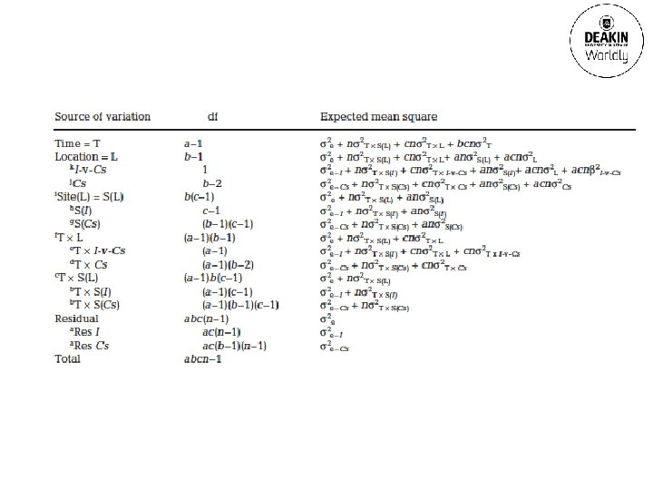
Impact assessment • Does sessile marine animal community composition vary between sewage impact and control sites? – 3 control and 1 impact locations – 4 randomly chosen times – replicate sites and photographic quadrats at each location • Percent cover of 58 taxa • Classical “beyond” BACI design – split-plot type linear model • Terlizzi et al (2005) http: //www. conisma. it/total/t_aim. html

Three broad approaches • Eigenanalyses – distance measure implied • Distance-based analyses – distance measure explicit and user-selected • Multi-species linear models – combine taxon-specific univariate (linear) models – no distance measure required

Eigenanalysis methods • Principal components analysis (PCA) – implied Euclidean distance • Correspondence analysis (CA) – implied chi-square distance • Canonical correspondence analysis (CCA/CANOCO) – constrains ordination based on linear modelling with environmental variables • Strengths – biplots of sample and species ordinations – CCA provides measures of fit with covarying environmental variables Cajo ter Braak

Rodents in habitat fragments SITE Florida Sandmark 34 street Balboaterr Katesess Altalajolla Laurel Canon Zena etc. AREA 25 84. 1 53. 8 51. 8 25. 6 32. 1 9. 7 8. 5 DISTX AGE 2100 914 1676 243 822 121 1554 1219 2865 Bolger et al (1997) 50 20 34 34 16 14 79 58 36 RRATTUS MMUS 0 0 0 0 3 PCALIF 13 1 4 4 2 1 11 16 8 PEREM 3 57 36 53 63 48 0 0 0 1 65 0 1 21 35 0 0 0 RMEGAL NFUSC NLEPID 1 2 9 16 2 9 5 30 11 16 12 8 0 0 0 0 8 0 0 0 12 0 0 0 PFALLAX MCALIF 0 2 0 18 0 2 0 0 3 0 2 0 0 0

Rodent data – CA biplot Axis 2 Rr Acuna El mac 54 th Street Baja Zena 32 nd Street Sth Oakcrest Axis 1 Florida Mm 7 fragments

Rodent data – CCA triplot Axis 2 Mc Pe Sandmark Nl Area 34 th Street Balboa Mm Dist Laurel Spruce Age Axis 1 Edison Acuna 54 th Street El mac Montanosa Rr

Issues • Both methods “compress” distances at ends of axes (socalled arch or horseshoe effect) Comp 2 – detrended CA brute force “fix” for this effect • CA and CCA implicitly upweight rarer taxa by use of chi -square distance • No choice of distance measure Comp 1 PCA bird community data

Distance-based methods • Include principal coordinates analysis (PCo. A), multidimensional scaling (MDS), generalised dissimilarity modelling (GDS) • Hypothesis testing – compare groups using multi-response permutation procedure (MRPP), analysis of similarities (ANOSIM), permutational multivariate ANOVA (PERMANOVA) – relate to environmental variables with Mantel test, BIO-ENV Marti Anderson John Curtis Bob Clarke

Distance-based methods • Strengths – flexibility of distance/dissimilarity measure, standardisation and transformation – consistency in that ordination and subsequent analyses based on original dissimilarities – some dissimilarities can be “decomposed” into relative taxon contributions (similarity percentages - SIMPER)

n. MDS – bird community data

PERMANOVA – bird community data

n. MDS – subtidal reef data

PERMANOVA – subtidal reef data

Issues • Flexible choice of distance/dissimilarity measure – ecologists nearly always default to Bray-Curtis – does B-C represent ecological differences of interest? • Modelling dissimilarities tricky – appropriate probability distributions – permutation procedures usually applied – robustness for complex models? – PERMANOVA only partitions SS not likelihoods – lack of independence – rely on permutation robustness • Limited predictive capacity • Distance-based methods cannot easily separate location and dispersion effects

• Location vs dispersion • Warton et al (2012)

Location vs dispersion • Transformation of abundances may help BUT many taxa have very skewed distributions • Issue recognised by PRIMER/PERMANOVA – “we can consider the homogeneity of dispersions to be included as part of the general null hypothesis of "no differences" among groups being tested by PERMANOVA (even though the focus of the PERMANOVA test is to detect location effects)” (PERMANOVA manual p. 22) • On going debate PRIMER/PERMANOVA vs mvabund

“Univariate” linear model approach • Fit separate generalised linear models to each taxon – based on –ve binomial distribution (over-dispersed counts) • Testing overall group or covariate effects – sum likelihood ratio (LR) tests across taxa – use permutation (resampling) methods to generate test statistic • Relative taxon contribution to patterns – LR statistic as measure of strength of individual taxon contributions • Strengths – linear models framework, univariate predictive capacity – handles mean-variance relationship • Issues – not an “ordination” method David Warton

Methods in community ecology • Journals searched 2011 -2012 – Austral Ecology – Oikos • Analyses of community/assemblage (species abundance incl. pres-abs data) – 62 papers found • Methods used – – – overall multivariate “philosophy” choice of dissimilarity measure (if relevant) transformation/standardisation used modeling (hypothesis testing) method choice of “ordination” plot

Multivariate approach Approach Eigenanalysis Distance-based Combined taxonspecific linear models # papers 15 47 0 % papers 24 76 0

Eigenanalyses Approach MANOVA / DFA PCA Correspondence analysis (incl. detrended) Constrained (canonical) correspondence analysis # papers 3 0 8 4 Majority of “ordinations” based on biplots, many with vectors fitted for environmental predictors (triplots)

Distance-based Dissimilarity measure Bray-Curtis Sorensen Jaccard Gower # papers 31 4 2 2

Distance/dissimilarity • Why do ecologists default to Bray-Curtis? – Faith et al (1987 – Vegetatio) strongly recommended B-C as robust indicator of ecological gradients – ranges between 0 (identical samples) and 1 (no species in common) – handles joint absences (taxa missing from both samples) – default in PRIMER/PERMANOVA, PC-ORD • Does B-C represent patterns ecologists are really interested in?

Distance-based Approach Comparing groups ANOSIM / PERMANOVA / db. RDA MRPP ANOVA on MDS axis scores # papers 24 6 2 Majority of “ordinations” based on non-metric MDS, 3 papers used cluster analysis

Distance-based Approach Relating to env predictors BIO-ENV/ Relate Mantel tests Regression/correlation with MDS axis scores Generalised dissimilarity modelling Determining taxa driving group differences SIMPER # papers 24 6 2 1 9

Transformations • Transformations of abundances common in ecology – log (y+1) or square/fourth root – original PRIMER program had 4 th root as default! • Most common reason - to reduce the influence of most abundant (dominant) taxa and give relatively greater weighting to rarer taxa – each taxon will be affected differently depending on its distribution? – effects on interaction terms almost never considered • Issues of unequal dispersions almost never raised in ecological papers – “it is not at all difficult to understand that transformations will also affect relative dispersions in multivariate space” (PERMANOVA manual p. 97)

Standardisations None Sample • Invertebrate assemblages in lake (Quinn et al 1996) • Four site-season combinations • n. MDS on Bray-Curtis • Four standardisations: • • None By sample totals By taxa totals Double • Bray-Curtis vs Canberra Taxa Double

To Bayes or not to Bayes….

Bayesian approaches • Detecting transitions between upslope and riparian vegetation – management of stream riparian zones • Based on plant assemblage data (% cover) along transects away from stream – pairwise Canberra distances between quadrats along each transect • Aim - to find the model with the highest probability of being the break between riparian and upslope vegetation – usual MCMC estimation of models Acheron River

Bayes factors > 10 Higher elevation sites Lower elevation sites Mac Nally et al (2008) Plant Ecology

Bayesian approaches • Maybe more robust than ML for complex models – already being used for variance estimation and confidence (credible) intervals in some mixed model software • Straightforward(? ) under mvabund generalised linear model approach – select suitable probability distributions for parameters – use uninformative prior if appropriate • More difficult with distance-based methods – but can be adapted (see Mac Nally 2005 Divers & Distr) – other examples using MDS and clustering (Oh & Raftery 2007 J Comp Graph Stat) focus on graphical representation (“ordination”)

Questions for discussion • Is the confounding of location and dispersion a “fatal” flaw for distance-based measures? – more direct comparisons between distance-based and linear model approaches needed • Comparison to other new methods – generalised dissimilarity modelling (Ferrier et al 2007) – gradient forests (Ellis et al 2012) • If distance-based measures are used: – what does Bray-Curtis actually measure ecologically? • What do multivariate models actually predict?

Questions for discussion • Should ecologists re-think their use of transformations? – NOT just a multivariate issue! • How do ecologists determine optimum sample sizes for community ecology – power characteristics will vary between taxa in linear models approach – power for distance-based permutation analyses?