Multivariate Analysis And PCA 1 Principal Components Analysis








- Slides: 83

Multivariate Analysis And PCA 1

Principal Components Analysis ( PCA) • Is a Factor Analytic method • Can be used to: – Reduce number of dimensions in data – Find patterns in high-dimensional data – Visualize data of high dimensionality • Example applications: – Face recognition – Image compression – Gene expression analysis 2

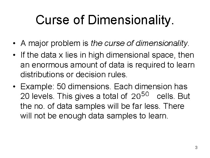
Curse of Dimensionality. • A major problem is the curse of dimensionality. • If the data x lies in high dimensional space, then an enormous amount of data is required to learn distributions or decision rules. • Example: 50 dimensions. Each dimension has 20 levels. This gives a total of cells. But the no. of data samples will be far less. There will not be enough data samples to learn. 3

What is PCA(Principal Component Analysis) • Basic idea : Given the data in M-Space, PCA reduce the dimensionality of a data set in which there a large number of interrelated variables , while retaining as much as possible of the variation present in the data set. This can be achieved by transforming to a new set of variables, the principle components, which are uncorrelated and are order so that the first few retain most of the variation present in all of the original variables 4

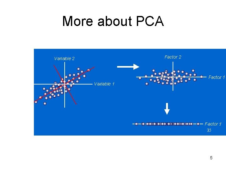
More about PCA 5

Benefits of PCA • Reduction of computation and storage overhead • Reduction of noise • Useful for visualizing the data 6

Multivariate Analysis: Multiple Regression Ordination 7

Ordination Goal: to discover and summarize the main patterns of variation in a set of variables measured over a number of sample locations. 8

Ordination techniques may generate useful simplifications of patterns in complex multivariate data sets. § Ordination combine common variation into new variables (multivariate axes) along which samples are ordered. § 9

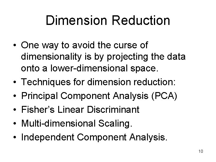
Dimension Reduction • One way to avoid the curse of dimensionality is by projecting the data onto a lower-dimensional space. • Techniques for dimension reduction: • Principal Component Analysis (PCA) • Fisher’s Linear Discriminant • Multi-dimensional Scaling. • Independent Component Analysis. 10

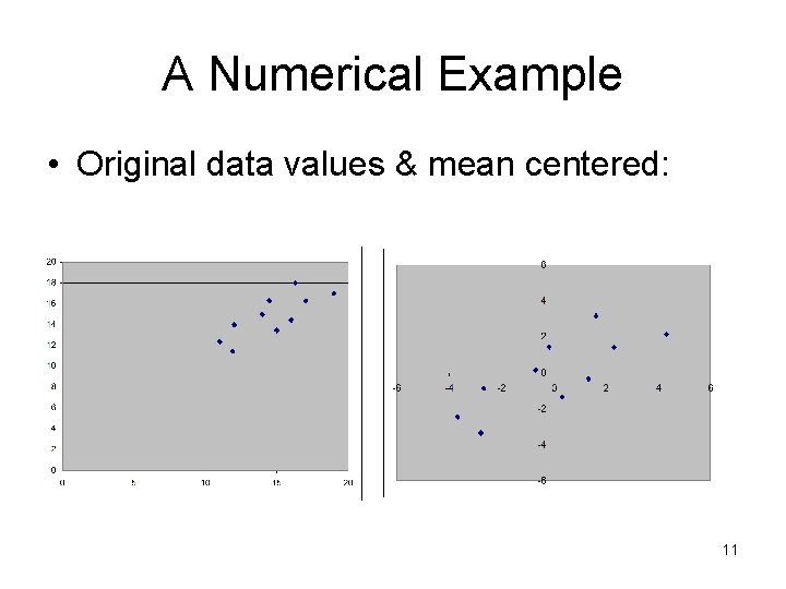
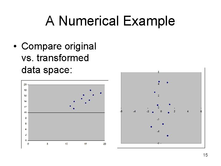
A Numerical Example • Original data values & mean centered: 11

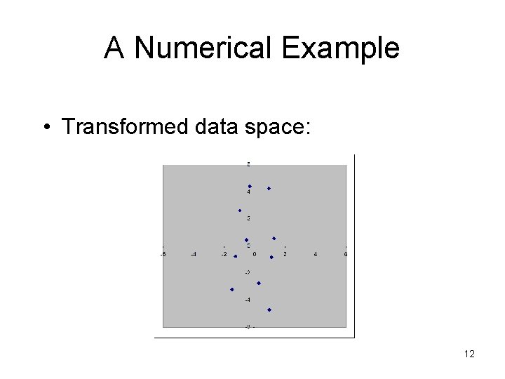
A Numerical Example • Transformed data space: 12

Ordination “A procedure for adapting a multidimensional swarm of data points in such a way that when it is projected onto a reduced number of dimensions any intrinsic pattern will become apparent” 13

Ordination Data reduction technique: §To select low-dimensional projections of the data for graphing. §To search for “structure” in the data. 14

A Numerical Example • Compare original vs. transformed data space: 15

Ordination methods: Principal Component Analysis (PCA) § Correspondence Analysis (CA) § Principal Coordinate Analysis (PCo. A) § Discriminant Function Analysis (DFA) § 16

PCA: Principal components analysis (PCA) is perhaps the most common technique used to summarize patterns among variables in multivariate datasets. 17

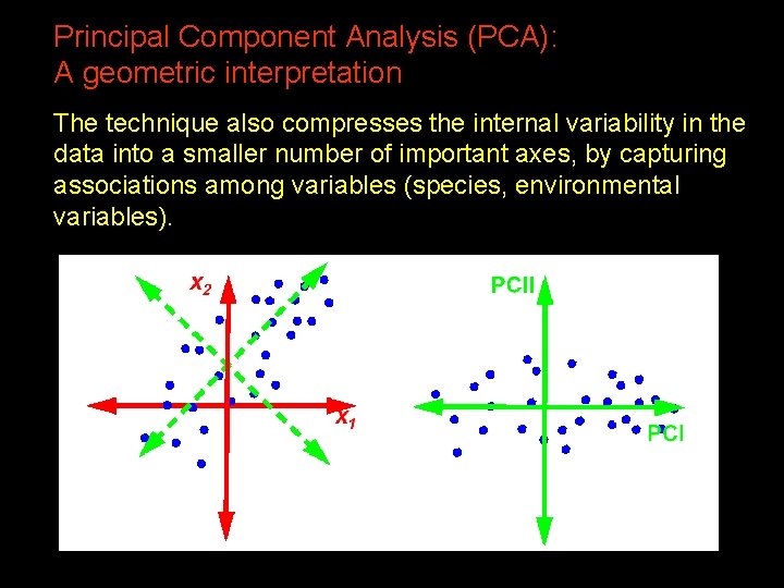
Principal Component Analysis (PCA): A geometric interpretation PCA constructs a new coordinate system new variables - which are linear combinations of the original axes and which are defined to align the samples along their major dimensions or axes of variation. § §PCA finds the coordinate system that best represents the internal variability in the data, essentially representing the data. 18

Principal Component Analysis (PCA): A geometric interpretation The technique also compresses the internal variability in the data into a smaller number of important axes, by capturing associations among variables (species, environmental variables). 19

Basics & Background • Objective: Conceptualize underlying pattern or structure of observed variables yi 1, …, yip on p attributes at each of n sites si. • PCA can be viewed as a rotation between data spaces of yi 1, …, yip and ui 1, …, uip. • Where u 1 is measured along the direction of maximum separation (i. e. , variance) and u 2 along the second in line and so forth … 20

Principal components • 1. principal component (PC 1) – the direction along which there is greatest variation • 2. principal component (PC 2) – the direction with maximum variation left in data, orthogonal to the 1. PC General about principal components – linear combinations of the original variables – uncorrelated with each other 21

Principal components 22

Basics & Background • Eigenvalue and Eigenvector: – Eigen originates in the German language and can be loosely translated as “of itself” – Thus an Eigenvalue of a matrix could be conceptualized as a “value of itself” – Eigenvalues and Eigenvectors are utilized in a wide range of applications (PCA, calculating a power of a matrix, finding solutions for a system of differential equations, and growth 23 models)

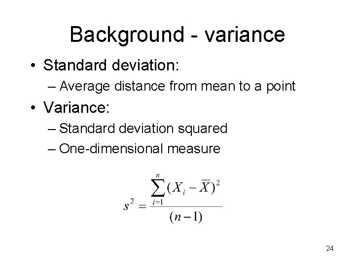
Background - variance • Standard deviation: – Average distance from mean to a point • Variance: – Standard deviation squared – One-dimensional measure 24

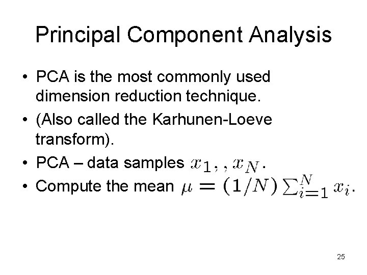
Principal Component Analysis • PCA is the most commonly used dimension reduction technique. • (Also called the Karhunen-Loeve transform). • PCA – data samples • Compute the mean 25

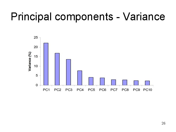
Principal components - Variance 26

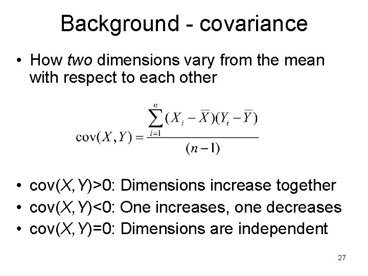
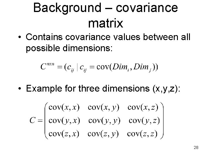
Background - covariance • How two dimensions vary from the mean with respect to each other • cov(X, Y)>0: Dimensions increase together • cov(X, Y)<0: One increases, one decreases • cov(X, Y)=0: Dimensions are independent 27

Background – covariance matrix • Contains covariance values between all possible dimensions: • Example for three dimensions (x, y, z): 28

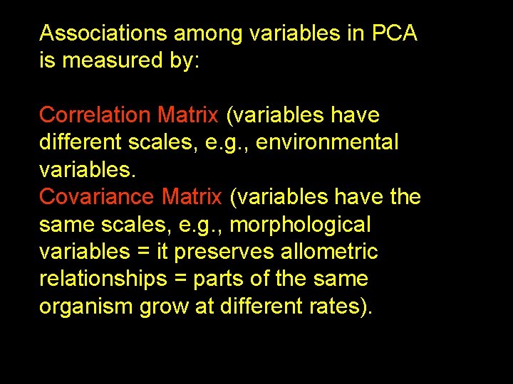
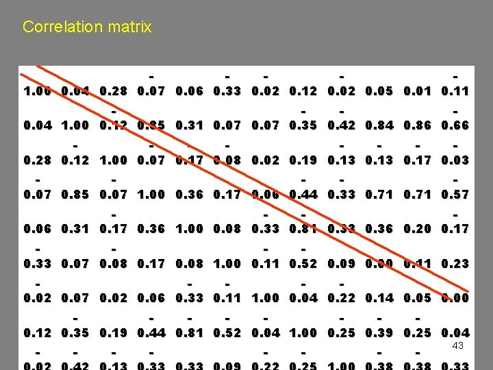
Associations among variables in PCA is measured by: Correlation Matrix (variables have different scales, e. g. , environmental variables. Covariance Matrix (variables have the same scales, e. g. , morphological variables = it preserves allometric relationships = parts of the same organism grow at different rates). 29

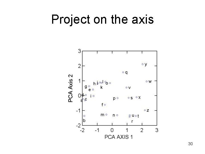
Project on the axis 30

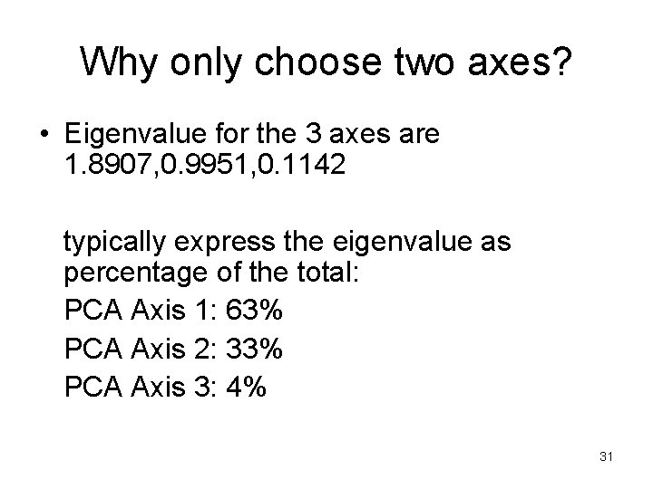
Why only choose two axes? • Eigenvalue for the 3 axes are 1. 8907, 0. 9951, 0. 1142 typically express the eigenvalue as percentage of the total: PCA Axis 1: 63% PCA Axis 2: 33% PCA Axis 3: 4% 31

Describing Video via PCA • Strategy: condense local spatial information using the PCA, and to preserve the temporal information by keeping all such reduced spatial information for all frames. 32

The mathematic of Principal Component Analysis (PCA): Eigenanalysis is a mathematical operation on a square, symmetric matrix (e. g. , pairwise correlation matrix). A square matrix has # rows =#cols. A symmetric matrix is transpose invariant. 33

The mathematic of Principal Component Analysis (PCA): The answer to an eigenanalysis consists of a series of eigenvalues and eigenvectors. Each eigenvalue has an eigenvector, and there as many eigenvectors and eigenvalues as there are rows in the initial correlation or covariance matrix. Eigenvalues are usually ranked from the greatest to the least. 34

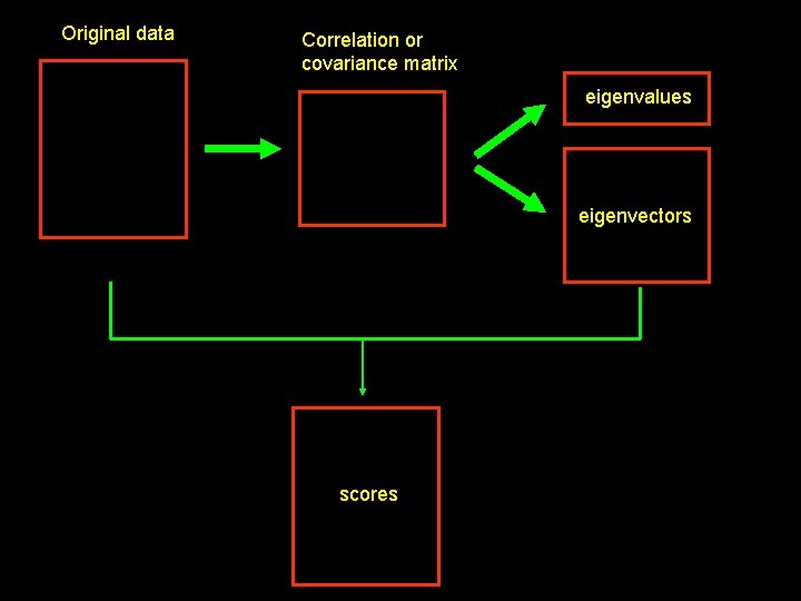
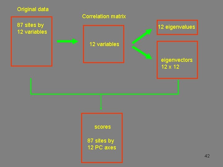
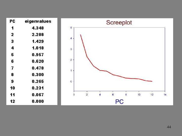
Principal component analysis presents three important structures: 1 - Eigenvalues: represent the amount of variation summarized by each principal component. The first principal component (PC -1) presents the largest amount, PC-2 presents the second largest, and so on. 35

Step 1 Extracting features • Features used in video analysis: color, texture, shape, motion vector… • Criteria of choosing features : they should have similar statistical behavior across time • Color histogram: simple and robust • Motion vectors: invariance to color and light 36

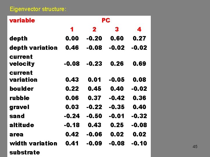
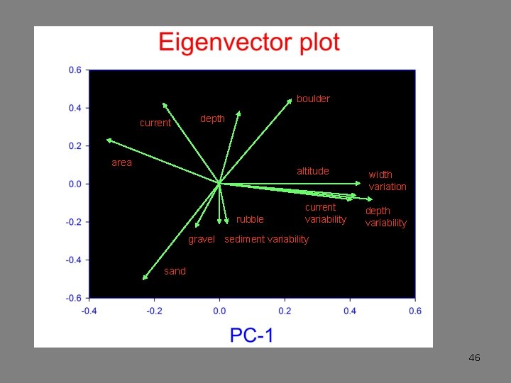
Principal component analysis presents three important structures: 2 - Eigenvectors: Each principal component is a linear function with coefficients for each variable. Eigenvectors contain these coefficients. High values, positive or negative, represents high association with the component. 37

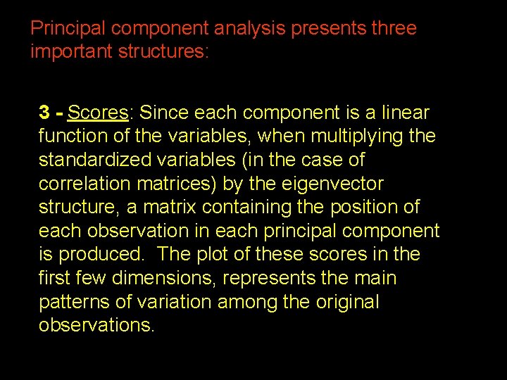
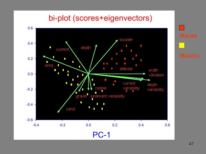
Principal component analysis presents three important structures: 3 - Scores: Since each component is a linear function of the variables, when multiplying the standardized variables (in the case of correlation matrices) by the eigenvector structure, a matrix containing the position of each observation in each principal component is produced. The plot of these scores in the first few dimensions, represents the main patterns of variation among the original observations. 38

Original data Correlation or covariance matrix eigenvalues eigenvectors scores 39

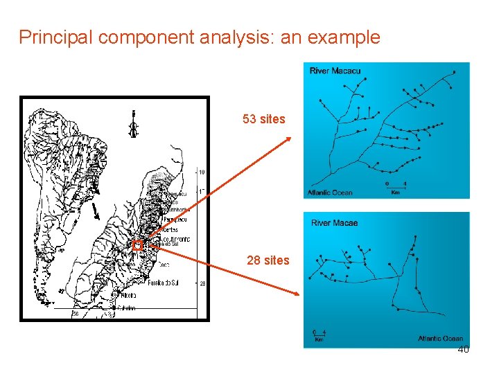
Principal component analysis: an example 53 sites 28 sites 40

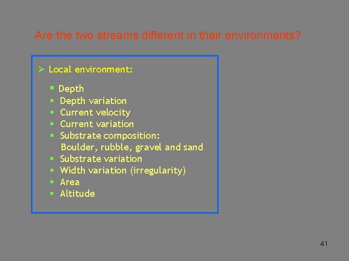
Are the two streams different in their environments? Ø Local environment: § Depth § § § § Depth variation Current velocity Current variation Substrate composition: Boulder, rubble, gravel and sand Substrate variation Width variation (irregularity) Area Altitude 41

Original data Correlation matrix 87 sites by 12 variables 12 eigenvalues 12 variables eigenvectors 12 x 12 scores 87 sites by 12 PC axes 42

Correlation matrix 1. 00 0. 04 0. 28 0. 07 0. 06 0. 33 0. 02 0. 12 0. 05 0. 01 0. 11 0. 04 1. 00 0. 12 0. 85 0. 31 0. 07 0. 35 0. 42 0. 84 0. 86 0. 66 0. 28 0. 12 1. 00 0. 07 0. 17 0. 08 0. 02 0. 19 0. 13 0. 17 0. 03 0. 07 0. 85 0. 07 1. 00 0. 36 0. 17 0. 06 0. 44 0. 33 0. 71 0. 57 0. 06 0. 31 0. 17 0. 36 1. 00 0. 08 0. 33 0. 81 0. 33 0. 36 0. 20 0. 17 0. 33 0. 07 0. 08 0. 17 0. 08 1. 00 0. 11 0. 52 0. 09 0. 00 0. 11 0. 23 0. 02 0. 07 0. 02 0. 06 0. 33 0. 11 1. 00 0. 04 0. 22 0. 14 0. 05 0. 00 0. 12 0. 35 0. 19 0. 44 0. 81 0. 52 0. 04 1. 00 0. 25 0. 39 0. 25 0. 04 - - - - 43

PC eigenvalues 1 4. 348 2 2. 288 3 1. 429 4 1. 018 5 0. 957 6 0. 620 7 0. 478 8 0. 300 9 0. 265 10 0. 231 11 0. 067 12 0. 000 44

Eigenvector structure: variable PC 1 2 3 4 depth 0. 00 -0. 20 0. 60 0. 27 depth variation 0. 46 -0. 08 -0. 02 current velocity -0. 08 -0. 23 0. 26 0. 69 current variation 0. 43 0. 01 -0. 05 0. 08 boulder 0. 22 0. 45 0. 40 -0. 02 rubble 0. 06 0. 37 -0. 42 0. 36 gravel 0. 03 -0. 22 -0. 35 0. 40 sand -0. 24 -0. 50 -0. 01 -0. 32 altitude -0. 18 0. 43 0. 25 -0. 08 area 0. 42 -0. 06 0. 02 width variation 0. 41 -0. 09 -0. 08 -0. 10 substrate 45

boulder current depth area altitude rubble current variability width variation depth variability gravel sediment variability sand 46

Macae boulder current depth Macacu area altitude rubble current variability width variation depth variability gravel sediment variability sand 47

Ordination bi-plots This summary is often a useful end in itself: the analysis discovers the latent structure of the data and how the variables contribute to this structure. 48

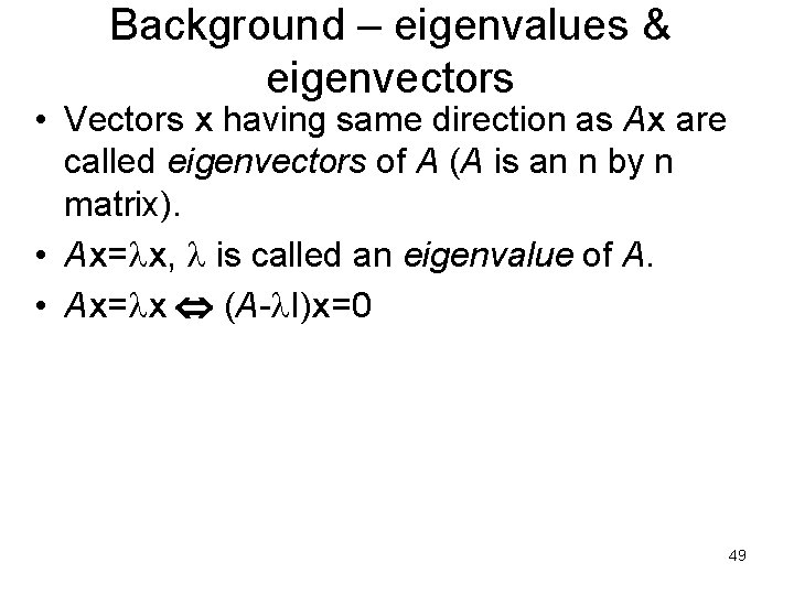
Background – eigenvalues & eigenvectors • Vectors x having same direction as Ax are called eigenvectors of A (A is an n by n matrix). • Ax= x, is called an eigenvalue of A. • Ax= x (A- I)x=0 49

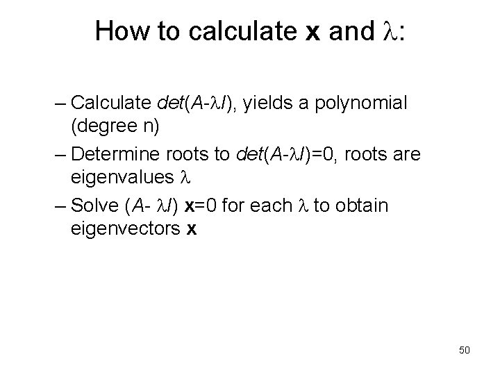
How to calculate x and : – Calculate det(A- I), yields a polynomial (degree n) – Determine roots to det(A- I)=0, roots are eigenvalues – Solve (A- I) x=0 for each to obtain eigenvectors x 50

PCA – step 1 • Get some data! – The data is organized as a matrix Data – Rows are observations – Columns are dimensions (variables) – Observations can also act as dimensions and vice versa by transposing matrix 51

Color Example • • • Let pixel p 1 be r 1, g 1, b 1 A ={P 1, P 2, P 3} D 1={r 1, r 2, r 3} D 2={g 1, g 2, g 3} D 3={b 1, b 2, b 3} Why use RGB? If you want skin tones, why not use IYQ? 52

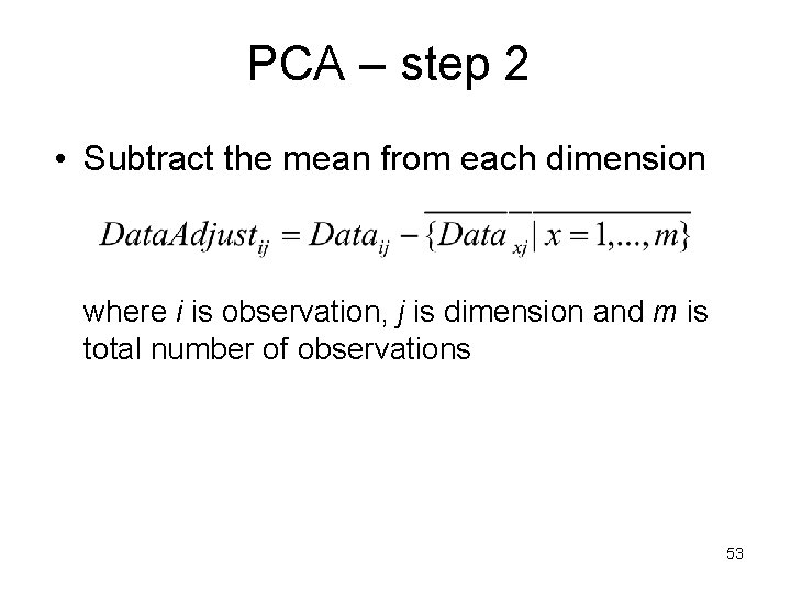
PCA – step 2 • Subtract the mean from each dimension where i is observation, j is dimension and m is total number of observations 53

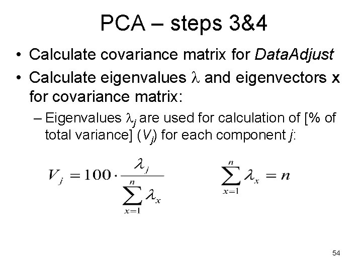
PCA – steps 3&4 • Calculate covariance matrix for Data. Adjust • Calculate eigenvalues and eigenvectors x for covariance matrix: – Eigenvalues j are used for calculation of [% of total variance] (Vj) for each component j: 54

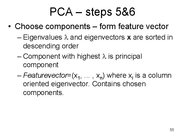
PCA – steps 5&6 • Choose components – form feature vector – Eigenvalues and eigenvectors x are sorted in descending order – Component with highest is principal component – Featurevector=(x 1, . . . , xn) where xi is a column oriented eigenvector. Contains chosen components. 55

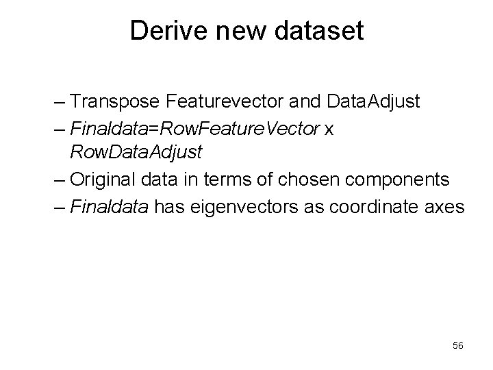
Derive new dataset – Transpose Featurevector and Data. Adjust – Finaldata=Row. Feature. Vector x Row. Data. Adjust – Original data in terms of chosen components – Finaldata has eigenvectors as coordinate axes 56

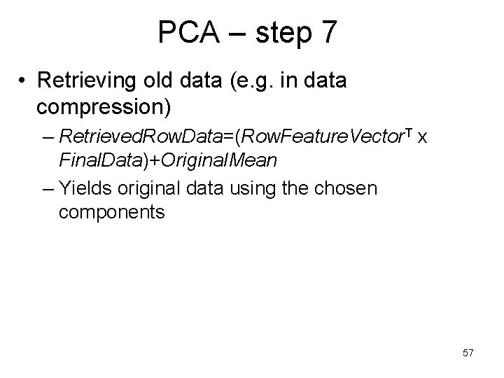
PCA – step 7 • Retrieving old data (e. g. in data compression) – Retrieved. Row. Data=(Row. Feature. Vector. T x Final. Data)+Original. Mean – Yields original data using the chosen components 57

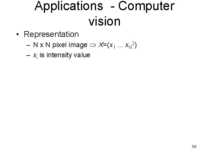
Applications - Computer vision • Representation – N x N pixel image X=(x 1. . . x. N 2) – xi is intensity value 58

PCA for Pattern identification – Perform PCA on matrix of M images – If new image Which original image is most similar? – Traditionally: difference original image and new image – PCA: difference PCA data and new image – Advantage: PCA data reflects similarities and differences in image data – Omitted dimensions still good performance 59

Applications – Computer vision • PCA for image compression – M images, each containing N 2 pixels – Dataset of M dimensions and N 2 observations – Corresponding pixels form vectors of intensities – PCA produces M eigenvectors and eigenvalues – Compress: choose limited number of components – Information loss when recreating original data 60

Motion Detection using PCA 61

Agenda n Motion Detection ¨ Input Video ¨ Algorithm Steps (2 -D and 3 -D blocks) ¨ Results n Sample Videos and Results ¨ Video with 8 x 8 Detection Blocks ¨ Video with 32 x 32 Detection Blocks 62

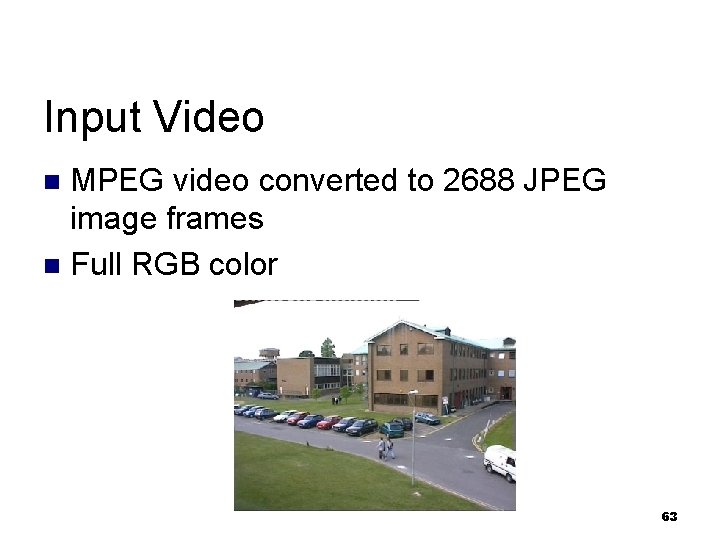
Input Video MPEG video converted to 2688 JPEG image frames n Full RGB color n 63

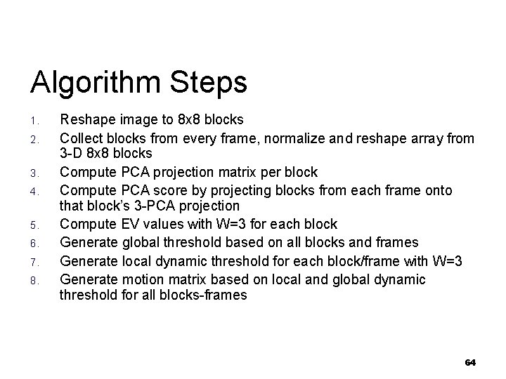
Algorithm Steps 1. 2. 3. 4. 5. 6. 7. 8. Reshape image to 8 x 8 blocks Collect blocks from every frame, normalize and reshape array from 3 -D 8 x 8 blocks Compute PCA projection matrix per block Compute PCA score by projecting blocks from each frame onto that block’s 3 -PCA projection Compute EV values with W=3 for each block Generate global threshold based on all blocks and frames Generate local dynamic threshold for each block/frame with W=3 Generate motion matrix based on local and global dynamic threshold for all blocks-frames 64

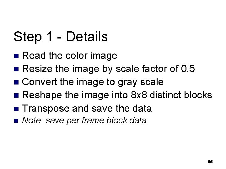
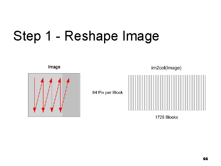
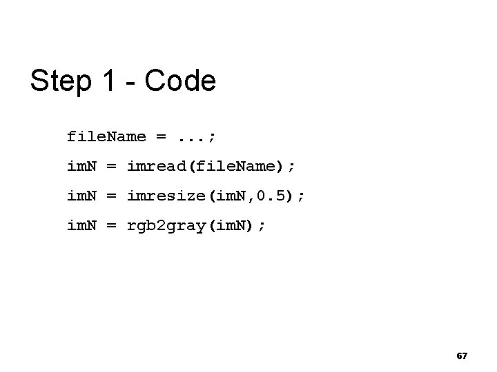
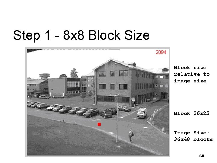
Step 1 - Details Read the color image n Resize the image by scale factor of 0. 5 n Convert the image to gray scale n Reshape the image into 8 x 8 distinct blocks n Transpose and save the data n n Note: save per frame block data 65

Step 1 - Reshape Image 66

Step 1 - Code file. Name =. . . ; im. N = imread(file. Name); im. N = imresize(im. N, 0. 5); im. N = rgb 2 gray(im. N); 67

Step 1 - 8 x 8 Block Size Block size relative to image size Block 26 x 25 Image Size: 36 x 48 blocks 68

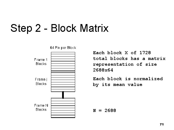
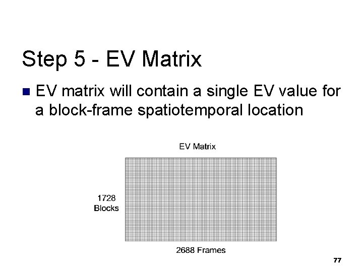
Step 2 - Collect Blocks n n n Collect same block from all the frames Create a single matrix for each block location Reshape vector from 3 -D 8 x 8 blocks There are 1728 matrices holding pixel values Each matrix is 2688 x 64 (frames x pixels/block) 69

Step 2 -Normalize Blocks Normalize each block by its mean value n Each block has its mean subtracted from each of the 64 pixel values n Store the normalized block data to be used in Step 3 and Step 4 n 70

Step 2 - Block Matrix Each block X of 1728 total blocks has a matrix representation of size 2688 x 64 Each block is normalized by its mean value N = 2688 71

Step 2 – 3 -D 8 x 8 Blocks Take 3 rows of Block matrix from previous slide 3 x 64 n Reshape into 1 x 192 vector n 3 -D blocks are overlapping n New 3 -D Block Matrix is used in computing PCA scores and projection matrices n 72

Step 3 - Compute PCA n Load normalized block matrix from Step 2 and compute the PCA projection matrix for this block sequence 73

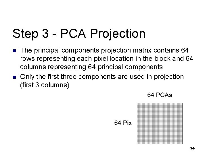
Step 3 - PCA Projection n n The principal components projection matrix contains 64 rows representing each pixel location in the block and 64 columns representing 64 principal components Only the first three components are used in projection (first 3 columns) 74

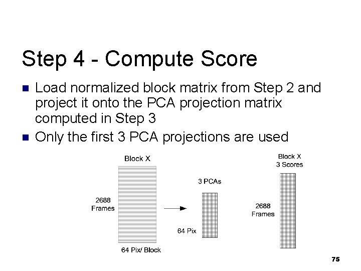
Step 4 - Compute Score n n Load normalized block matrix from Step 2 and project it onto the PCA projection matrix computed in Step 3 Only the first 3 PCA projections are used 75

Step 5 - Compute EV n n n For each block sequence, load the PCA score matrix computed in Step 4 Compute a covariance matrix using a moving window of size 3 Compute eigenvalues (EVs) Sort to get the larges EV value Store the data in one EV matrix, representing all blocks and all frames 76

Step 5 - EV Matrix n EV matrix will contain a single EV value for a block-frame spatiotemporal location 77

Step 6 - Global Threshold Load EV matrix from Step 5 n Compute mean and standard deviation n Find all entries in the EV matrix that are below mean+2*std n n Update the EV matrix 78

Step 7 - Local Threshold Use the updated EV matrix from Step 6 n Compute a local dynamic threshold using window n Generate a Motion matrix of same size as the EV matrix with a simple 0/1 values (1=motion) n 79

Step 7 - Assumptions n n Assume that first 100 frames have no detectable motion Compute mean and std of first 100 frames for each block Compute local threshold for each block using a moving window (W=3) Adjust local threshold, when no moving object is detected 80

Step 8 - Motion Matrix Motion matrix is of size 1728 x 2688, same size as the EV matrix n It contains values 0 or 1, where 1 = motion detected n Use the Motion matrix to create sample videos showing blocks where motion was detected n 81

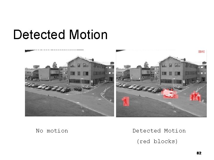
Detected Motion No motion Detected Motion (red blocks) 82

Conclusion The method of motion detection using principal component analysis combined with dynamic thresholding yields very good results in detecting motion n Future projects will include processing images with variation in size of the blocks n 83