Multivariate Analysis and Discrimination SPH 247 Statistical Analysis

Multivariate Analysis and Discrimination SPH 247 Statistical Analysis of Laboratory Data May 26, 2015 SPH 247 Statistical Analysis of Laboratory Data 1

Cystic Fibrosis Data Set �The 'cystfibr' data frame has 25 rows and 10 columns. It contains lung function data for cystic fibrosis patients (7 -23 years old) �We will examine the relationships among the various measures of lung function May 26, 2015 SPH 247 Statistical Analysis of Laboratory Data 2

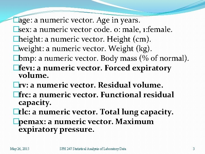
�age: a numeric vector. Age in years. �sex: a numeric vector code. 0: male, 1: female. �height: a numeric vector. Height (cm). �weight: a numeric vector. Weight (kg). �bmp: a numeric vector. Body mass (% of normal). �fev 1: a numeric vector. Forced expiratory volume. �rv: a numeric vector. Residual volume. �frc: a numeric vector. Functional residual capacity. �tlc: a numeric vector. Total lung capacity. �pemax: a numeric vector. Maximum expiratory pressure. May 26, 2015 SPH 247 Statistical Analysis of Laboratory Data 3

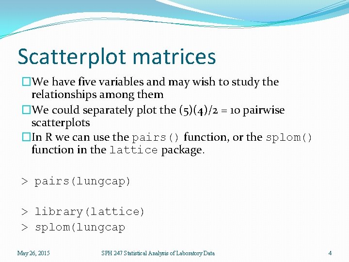
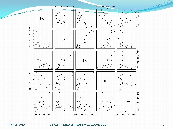
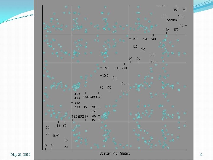
Scatterplot matrices �We have five variables and may wish to study the relationships among them �We could separately plot the (5)(4)/2 = 10 pairwise scatterplots �In R we can use the pairs() function, or the splom() function in the lattice package. > pairs(lungcap) > library(lattice) > splom(lungcap May 26, 2015 SPH 247 Statistical Analysis of Laboratory Data 4

May 26, 2015 SPH 247 Statistical Analysis of Laboratory Data 5

May 26, 2015 SPH 247 Statistical Analysis of Laboratory Data 6

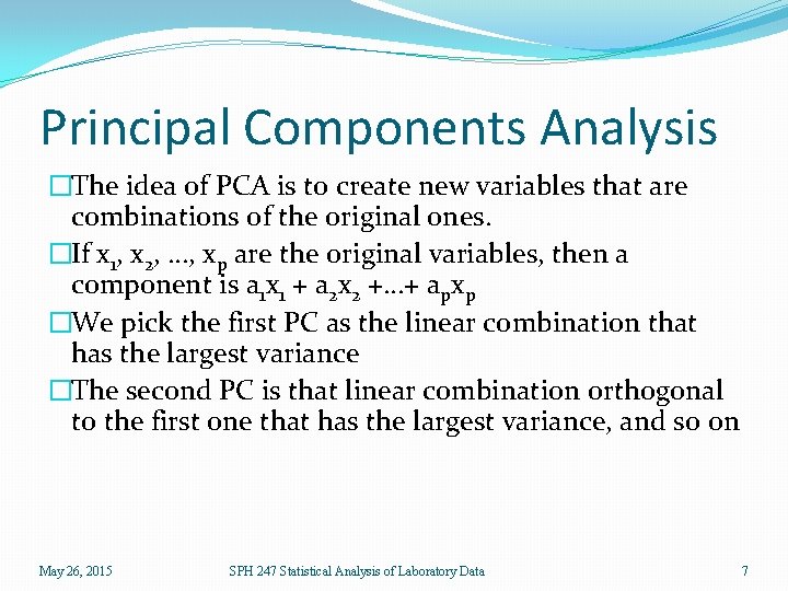
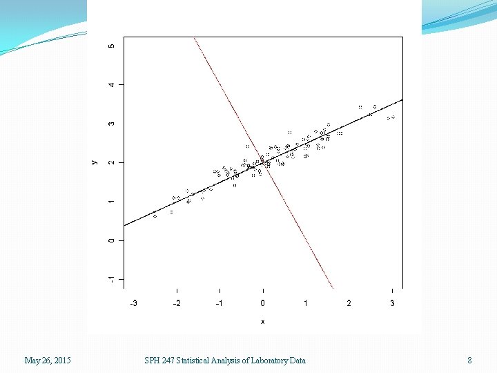
Principal Components Analysis �The idea of PCA is to create new variables that are combinations of the original ones. �If x 1, x 2, …, xp are the original variables, then a component is a 1 x 1 + a 2 x 2 +…+ apxp �We pick the first PC as the linear combination that has the largest variance �The second PC is that linear combination orthogonal to the first one that has the largest variance, and so on May 26, 2015 SPH 247 Statistical Analysis of Laboratory Data 7

May 26, 2015 SPH 247 Statistical Analysis of Laboratory Data 8

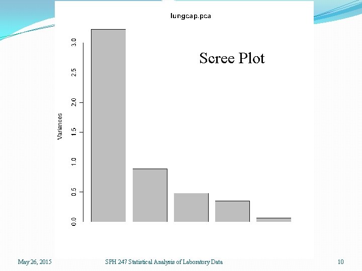
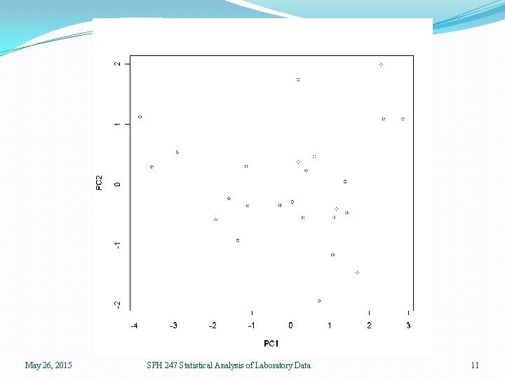
> lungcap. pca <- prcomp(lungcap, scale=T) > plot(lungcap. pca) > names(lungcap. pca) [1] "sdev" "rotation" "center" "scale" "x" > lungcap. pca$sdev [1] 1. 7955824 0. 9414877 0. 6919822 0. 5873377 0. 2562806 > lungcap. pca$center fev 1 rv frc tlc pemax 34. 72 255. 20 155. 40 114. 00 109. 12 > lungcap. pca$scale fev 1 rv frc tlc pemax 11. 19717 86. 01696 43. 71880 16. 96811 33. 43691 > plot(lungcap. pca$x[, 1: 2]) Always use scaling before PCA unless all variables are on the Same scale. This is equivalent to PCA on the correlation matrix instead of the covariance matrix May 26, 2015 SPH 247 Statistical Analysis of Laboratory Data 9

Scree Plot May 26, 2015 SPH 247 Statistical Analysis of Laboratory Data 10

May 26, 2015 SPH 247 Statistical Analysis of Laboratory Data 11

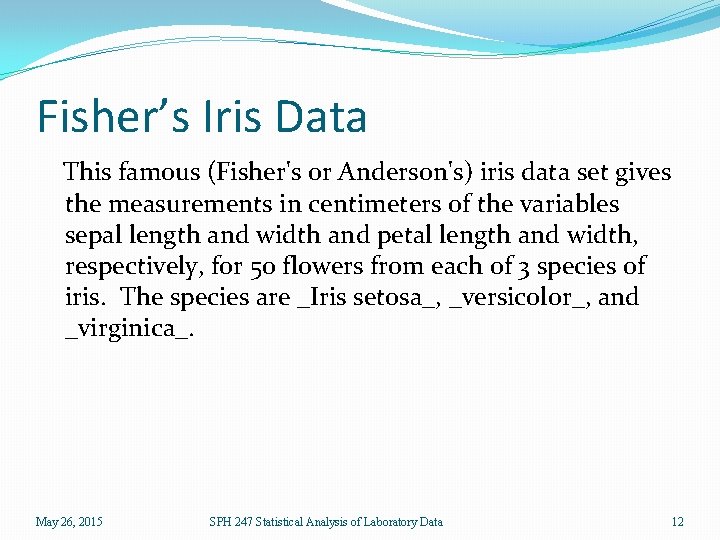
Fisher’s Iris Data This famous (Fisher's or Anderson's) iris data set gives the measurements in centimeters of the variables sepal length and width and petal length and width, respectively, for 50 flowers from each of 3 species of iris. The species are _Iris setosa_, _versicolor_, and _virginica_. May 26, 2015 SPH 247 Statistical Analysis of Laboratory Data 12

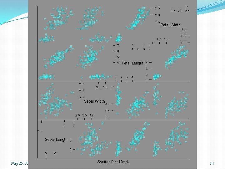
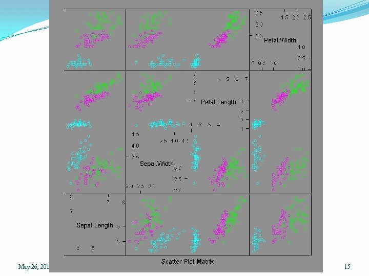
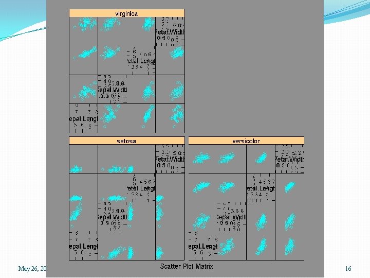
> data(iris) > help(iris) > names(iris) [1] "Sepal. Length" "Sepal. Width" > attach(iris) > iris. dat <- iris[, 1: 4] > splom(iris. dat) > splom(iris. dat, groups=Species) > splom(~ iris. dat | Species) > summary(iris) Sepal. Length Sepal. Width Min. : 4. 300 Min. : 2. 000 1 st Qu. : 5. 100 1 st Qu. : 2. 800 Median : 5. 800 Median : 3. 000 Mean : 5. 843 Mean : 3. 057 3 rd Qu. : 6. 400 3 rd Qu. : 3. 300 Max. : 7. 900 Max. : 4. 400 May 26, 2015 "Petal. Length" "Petal. Width" Petal. Length Min. : 1. 000 1 st Qu. : 1. 600 Median : 4. 350 Mean : 3. 758 3 rd Qu. : 5. 100 Max. : 6. 900 Petal. Width Min. : 0. 100 1 st Qu. : 0. 300 Median : 1. 300 Mean : 1. 199 3 rd Qu. : 1. 800 Max. : 2. 500 SPH 247 Statistical Analysis of Laboratory Data "Species" Species setosa : 50 versicolor: 50 virginica : 50 13

May 26, 2015 SPH 247 Statistical Analysis of Laboratory Data 14

May 26, 2015 SPH 247 Statistical Analysis of Laboratory Data 15

May 26, 2015 SPH 247 Statistical Analysis of Laboratory Data 16

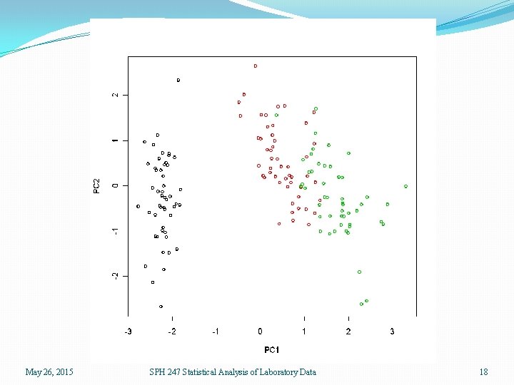
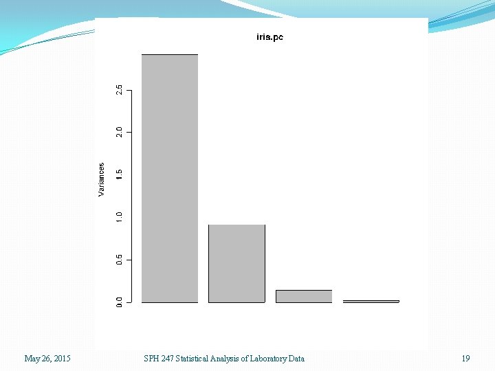
> data(iris) > iris. pc <- prcomp(iris[, 1: 4], scale=T) > plot(iris. pc$x[, 1: 2], col=rep(1: 3, each=50)) > names(iris. pc) [1] "sdev" "rotation" "center" "scale" "x" > plot(iris. pc) > iris. pc$sdev [1] 1. 7083611 0. 9560494 0. 3830886 0. 1439265 > iris. pc$rotation PC 1 PC 2 PC 3 PC 4 Sepal. Length 0. 5210659 -0. 37741762 0. 7195664 0. 2612863 Sepal. Width -0. 2693474 -0. 92329566 -0. 2443818 -0. 1235096 Petal. Length 0. 5804131 -0. 02449161 -0. 1421264 -0. 8014492 Petal. Width 0. 5648565 -0. 06694199 -0. 6342727 0. 5235971 May 26, 2015 SPH 247 Statistical Analysis of Laboratory Data 17

May 26, 2015 SPH 247 Statistical Analysis of Laboratory Data 18

May 26, 2015 SPH 247 Statistical Analysis of Laboratory Data 19

Discriminant Analysis �An alternative to logistic regression for classification is discrimininant analysis �This comes in two flavors, (Fisher’s) Linear Discriminant Analysis or LDA and (Fisher’s) Quadratic Discriminant Analysis or QDA �In each case we model the shape of the groups and provide a dividing line/curve May 26, 2015 SPH 247 Statistical Analysis of Laboratory Data 20

�One way to describe the way LDA and QDA work is to think of the data as having for each group an elliptical distribution �We allocate new cases to the group for which they have the highest likelihoods �This provides a linear cut-point if the ellipses are assumed to have the same shape and a quadratic one if they may be different May 26, 2015 SPH 247 Statistical Analysis of Laboratory Data 21

> library(MASS) > iris. lda <- lda(iris[, 1: 4], iris[, 5]) > iris. lda Call: lda(iris[, 1: 4], iris[, 5]) Prior probabilities of groups: setosa versicolor virginica 0. 3333333 Group means: Sepal. Length Sepal. Width Petal. Length Petal. Width setosa 5. 006 3. 428 1. 462 0. 246 versicolor 5. 936 2. 770 4. 260 1. 326 virginica 6. 588 2. 974 5. 552 2. 026 Coefficients of linear discriminants: LD 1 LD 2 Sepal. Length 0. 8293776 0. 02410215 Sepal. Width 1. 5344731 2. 16452123 Petal. Length -2. 2012117 -0. 93192121 Petal. Width -2. 8104603 2. 83918785 Proportion of trace: LD 1 LD 2 0. 9912 0. 0088 May 26, 2015 SPH 247 Statistical Analysis of Laboratory Data 22

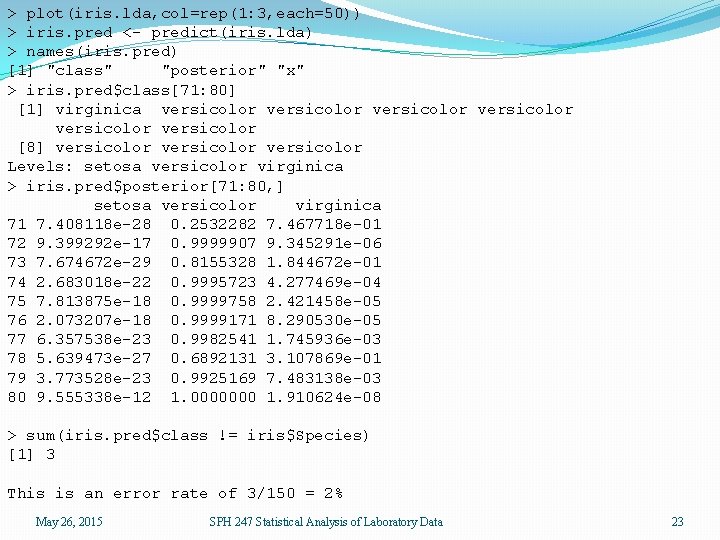
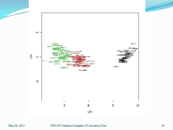
> plot(iris. lda, col=rep(1: 3, each=50)) > iris. pred <- predict(iris. lda) > names(iris. pred) [1] "class" "posterior" "x" > iris. pred$class[71: 80] [1] virginica versicolor versicolor [8] versicolor Levels: setosa versicolor virginica > iris. pred$posterior[71: 80, ] setosa versicolor virginica 71 7. 408118 e-28 0. 2532282 7. 467718 e-01 72 9. 399292 e-17 0. 9999907 9. 345291 e-06 73 7. 674672 e-29 0. 8155328 1. 844672 e-01 74 2. 683018 e-22 0. 9995723 4. 277469 e-04 75 7. 813875 e-18 0. 9999758 2. 421458 e-05 76 2. 073207 e-18 0. 9999171 8. 290530 e-05 77 6. 357538 e-23 0. 9982541 1. 745936 e-03 78 5. 639473 e-27 0. 6892131 3. 107869 e-01 79 3. 773528 e-23 0. 9925169 7. 483138 e-03 80 9. 555338 e-12 1. 0000000 1. 910624 e-08 > sum(iris. pred$class != iris$Species) [1] 3 This is an error rate of 3/150 = 2% May 26, 2015 SPH 247 Statistical Analysis of Laboratory Data 23

May 26, 2015 SPH 247 Statistical Analysis of Laboratory Data 24

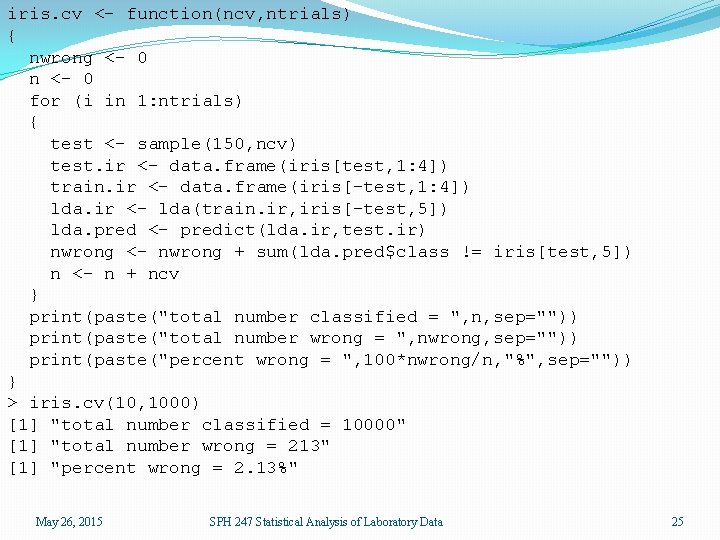
iris. cv <- function(ncv, ntrials) { nwrong <- 0 n <- 0 for (i in 1: ntrials) { test <- sample(150, ncv) test. ir <- data. frame(iris[test, 1: 4]) train. ir <- data. frame(iris[-test, 1: 4]) lda. ir <- lda(train. ir, iris[-test, 5]) lda. pred <- predict(lda. ir, test. ir) nwrong <- nwrong + sum(lda. pred$class != iris[test, 5]) n <- n + ncv } print(paste("total number classified = ", n, sep="")) print(paste("total number wrong = ", nwrong, sep="")) print(paste("percent wrong = ", 100*nwrong/n, "%", sep="")) } > iris. cv(10, 1000) [1] "total number classified = 10000" [1] "total number wrong = 213" [1] "percent wrong = 2. 13%" May 26, 2015 SPH 247 Statistical Analysis of Laboratory Data 25

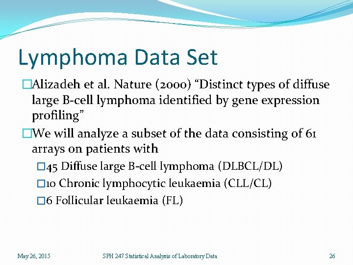
Lymphoma Data Set �Alizadeh et al. Nature (2000) “Distinct types of diffuse large B-cell lymphoma identified by gene expression profiling” �We will analyze a subset of the data consisting of 61 arrays on patients with � 45 Diffuse large B-cell lymphoma (DLBCL/DL) � 10 Chronic lymphocytic leukaemia (CLL/CL) � 6 Follicular leukaemia (FL) May 26, 2015 SPH 247 Statistical Analysis of Laboratory Data 26

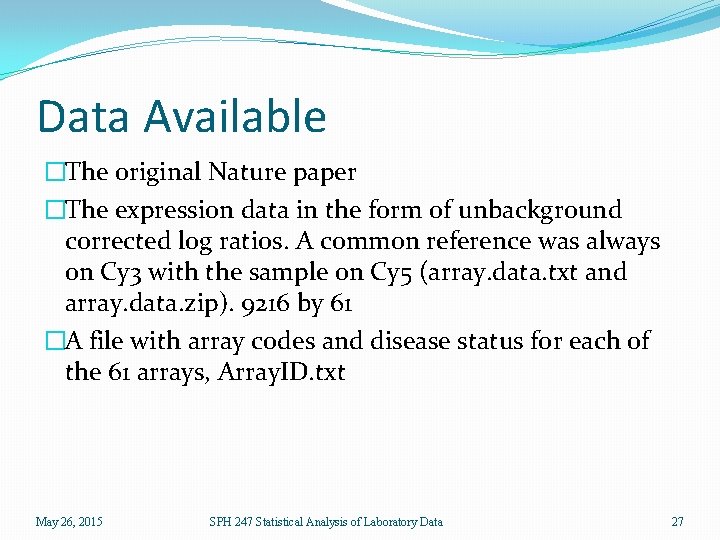
Data Available �The original Nature paper �The expression data in the form of unbackground corrected log ratios. A common reference was always on Cy 3 with the sample on Cy 5 (array. data. txt and array. data. zip). 9216 by 61 �A file with array codes and disease status for each of the 61 arrays, Array. ID. txt May 26, 2015 SPH 247 Statistical Analysis of Laboratory Data 27

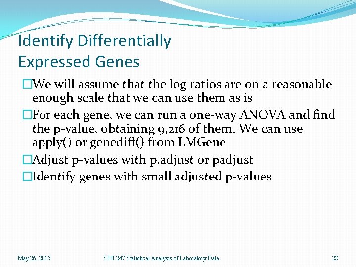
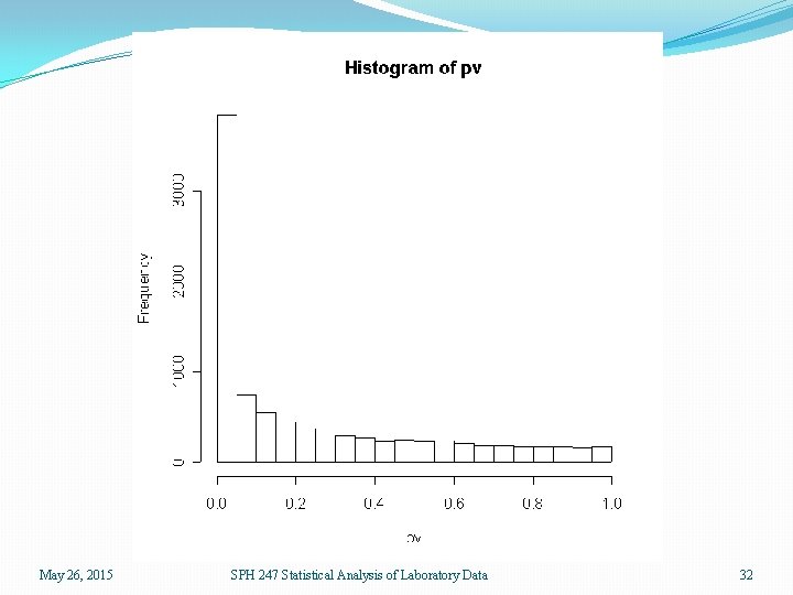
Identify Differentially Expressed Genes �We will assume that the log ratios are on a reasonable enough scale that we can use them as is �For each gene, we can run a one-way ANOVA and find the p-value, obtaining 9, 216 of them. We can use apply() or genediff() from LMGene �Adjust p-values with p. adjust or padjust �Identify genes with small adjusted p-values May 26, 2015 SPH 247 Statistical Analysis of Laboratory Data 28

Develop Classifier �Reduce dimension with ANOVA gene selection or with PCA. (We could also use stepwise logistic regression. ) �Use logistic regression or LDA. �Evaluate the four possibilities and their subpossibilities with cross validation. With 61 arrays one could reasonable omit 10% or 6 at random. May 26, 2015 SPH 247 Statistical Analysis of Laboratory Data 29

Differential Expression �We can locate genes that are differentially expressed; that is, genes whose expression differs systematically by the type of lymphoma. �To do this, we could use lymphoma type to predict expression, and see when this is statistically significant. �For one gene at a time, this is ANOVA. May 26, 2015 SPH 247 Statistical Analysis of Laboratory Data 30

�It is almost equivalent to locate genes whose expression can be used to predict lymphoma type, this being the reverse process. �If there is significant association in one direction there should logically be significant association in the other �This will not be true exactly, but is true approximately �We can also easily do the latter analysis using the expression of more than one gene using logistic regression, LDA, and QDA May 26, 2015 SPH 247 Statistical Analysis of Laboratory Data 31

May 26, 2015 SPH 247 Statistical Analysis of Laboratory Data 32

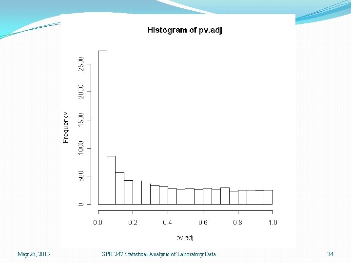
Significant Genes �There are 3845 out of 9261 genes that have significant p-values from the ANOVA of less than 0. 05, compared to 463 expected by chance �There are 2733 genes with FDR adjusted p-values less than 0. 05 �There are only 184 genes with Bonferroni adjusted pvalues less than 0. 05 May 26, 2015 SPH 247 Statistical Analysis of Laboratory Data 33

May 26, 2015 SPH 247 Statistical Analysis of Laboratory Data 34

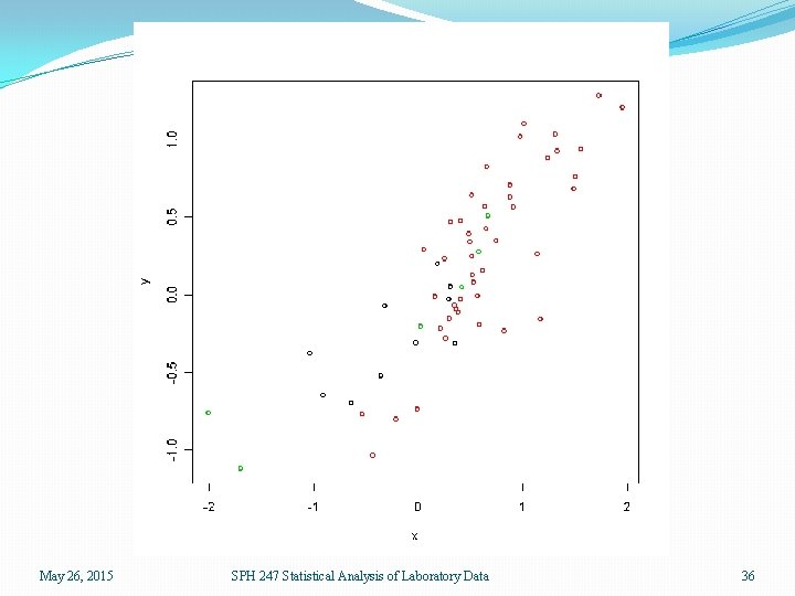
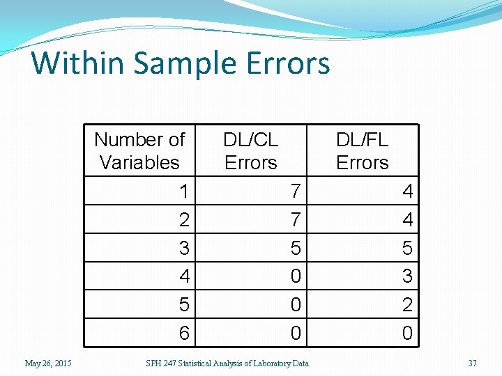
Logistic Regression �We will use logistic regression to distinguish DLBCL from CLL and DLBCL from FL �We will do this first by choosing the variables with the smallest overall p-values in the ANOVA �We will then evaluate the results within sample and by cross validation May 26, 2015 SPH 247 Statistical Analysis of Laboratory Data 35

May 26, 2015 SPH 247 Statistical Analysis of Laboratory Data 36

Within Sample Errors Number of Variables 1 2 3 4 5 6 May 26, 2015 DL/CL Errors DL/FL Errors 7 7 5 0 0 0 SPH 247 Statistical Analysis of Laboratory Data 4 4 5 3 2 0 37

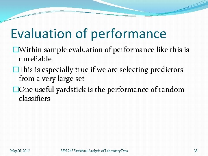
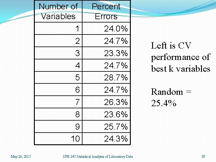
Evaluation of performance �Within sample evaluation of performance like this is unreliable �This is especially true if we are selecting predictors from a very large set �One useful yardstick is the performance of random classifiers May 26, 2015 SPH 247 Statistical Analysis of Laboratory Data 38

Number of Variables 1 2 3 4 5 6 7 8 9 10 May 26, 2015 Percent Errors 24. 0% 24. 7% 23. 3% 24. 7% 28. 7% 24. 7% 26. 3% 23. 6% 25. 7% 24. 3% SPH 247 Statistical Analysis of Laboratory Data Left is CV performance of best k variables Random = 25. 4% 39

Conclusion �Logistic regression on the variables with the smallest p-values does not work very well �This cannot be identified by looking at the within sample statistics �Cross validation is a requirement to assess performance of classifiers May 26, 2015 SPH 247 Statistical Analysis of Laboratory Data 40

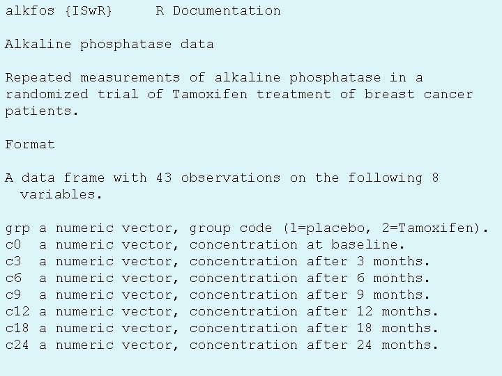
alkfos {ISw. R} R Documentation Alkaline phosphatase data Repeated measurements of alkaline phosphatase in a randomized trial of Tamoxifen treatment of breast cancer patients. Format A data frame with 43 observations on the following 8 variables. grp c 0 c 3 c 6 c 9 c 12 c 18 c 24 a a a a numeric numeric May 26, 2015 vector, vector, group code (1=placebo, 2=Tamoxifen). concentration at baseline. concentration after 3 months. concentration after 6 months. concentration after 9 months. concentration after 12 months. concentration after 18 months. concentration after 24 months. SPH 247 Statistical Analysis of Laboratory Data 41

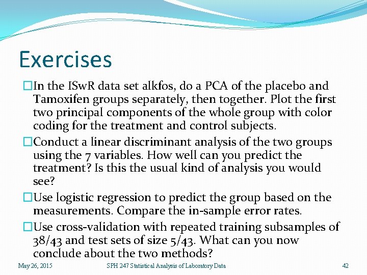
Exercises �In the ISw. R data set alkfos, do a PCA of the placebo and Tamoxifen groups separately, then together. Plot the first two principal components of the whole group with color coding for the treatment and control subjects. �Conduct a linear discriminant analysis of the two groups using the 7 variables. How well can you predict the treatment? Is this the usual kind of analysis you would see? �Use logistic regression to predict the group based on the measurements. Compare the in-sample error rates. �Use cross-validation with repeated training subsamples of 38/43 and test sets of size 5/43. What can you now conclude about the two methods? May 26, 2015 SPH 247 Statistical Analysis of Laboratory Data 42