Multispectral Image Classification Professor KeSheng Cheng Department of

Multispectral Image Classification Professor Ke-Sheng Cheng Department of Bioenvironmental Systems Engineering National Taiwan University

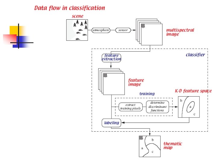
Thematic Maps or Images Multispectral images Thematic images n Themes (also known as classes) n Soil n Water n Vegetation n etc. n n Spectral signatures

The Classification Process Number and Types of classes n Extraction of classification features n Classification algorithms (classifiers) n Classification accuracy assessment n

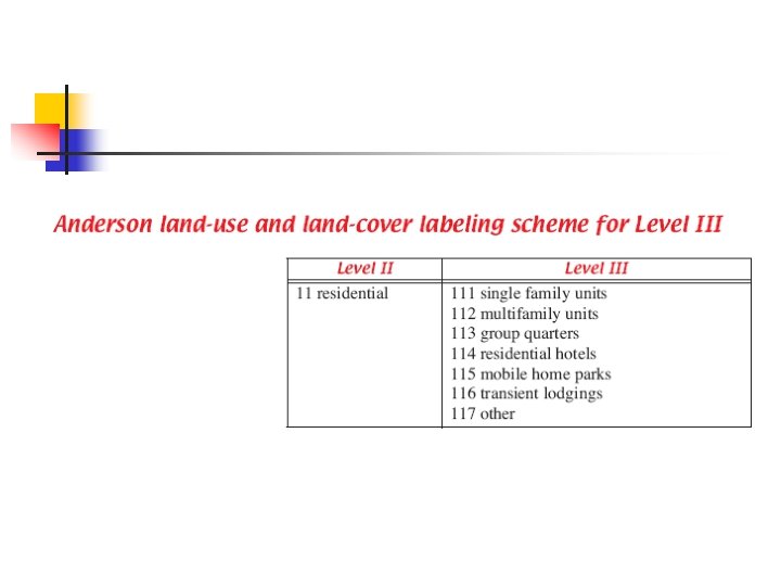
Land-use/Land-cover (LULC) Classes

Feature Extraction n Example features Original multispectral bands n Subset of bands n Derived features n Vegetation indices n Principal components n Textural features n

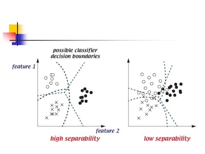
Feature Space Because of class variability, the “signature” is actually a statistical distribution of feature vectors. n Successful classification requires separated distributions, i. e. minimal overlap. n Image classification is essentially a work of feature space partition. n

Features Selection There may be many features available to us and we need to select “good” features to achieve high classification accuracies. n Separation index can be used to measure similarity or dissimilarity among classes. n

Types of Image Classification Algorithm n Classification processes Supervised classification n Unsupervised classification n n Characteristics of classification features Parametric classification n Nonparametric classification n

Supervised Classification n Collecting training data for each class. n Each training pixel is associated with a feature vector. Characterizing the feature pattern for each class from the training data. n Delineating class boundaries using mathematical or statistical methods. n Assigning pixels to corresponding classes. n

Supervised Classification in 2 -D Feature Space Satellite image to be classified Feature 2 Training data collection Delineating class boundaries Assigning classes to nontraining pixels Feature 1

Statistical Classification Algorithms Let X = (x 1, x 2, …, xn)T represent an ndimensional feature vector and 1, 2, …, M be M classes. We now define M decision (or discriminant) functions di(X), i=1, 2, …, M with the property that, if a pixel with feature vector X belongs to class i , then di(X) > dj(X), j=1, 2, …, M, i j.

n In the feature space, the decision boundary separating classes i and j is given by values of X which satisfies dij(X) = di(X) dj(X) = 0

Minimum Distance Classifier

We can also choose Thus, The decision boundary is

For minimum distance classifier, each class is characterized by its mean vector in the multidimensional feature space. n It does not consider the variance of each class. n

Maximum Likelihood Classifier

where fi(X) is the probability density function of feature vector of the class i. n For 1 -dimensional feature space and two classes case, it is equivalent to n The ML classifier does not consider the a priori probabilities of individual classes.

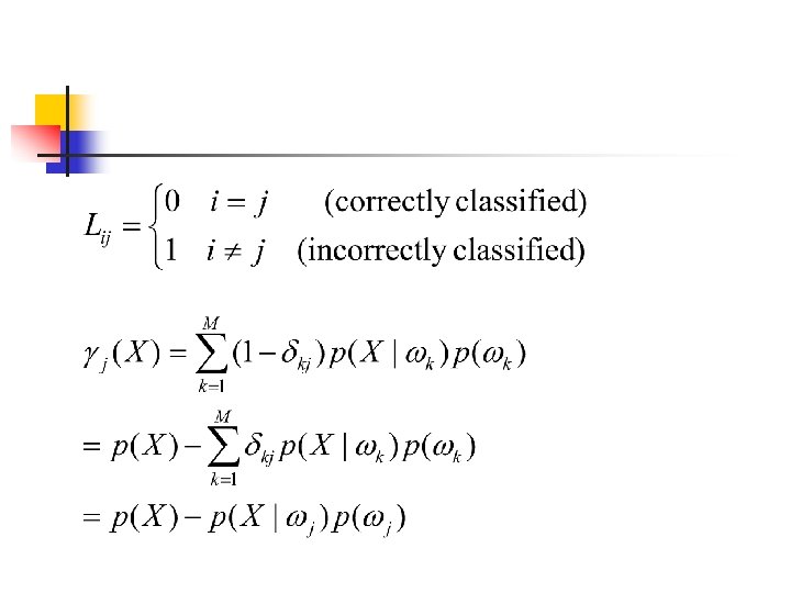
Bayes Classifier n n n Let the probability that a particular pixel with feature vector X comes from class i be denoted. If the classifier decides that the pixel comes from j when it actually comes from i, it incurs a loss, denoted Lij. However, the feature vector X may belong to any of the M classes under consideration, thus the average loss incurred in assigning X to j is :

n From the conditional probability

n n The decision for classification is Since p(X) is common for all j(X), we can also choose to use

n Therefore, n If we choose

n n Thus, the decision criterion for Bayes classifier is The decision function di(X) is

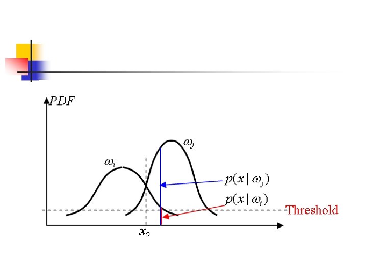
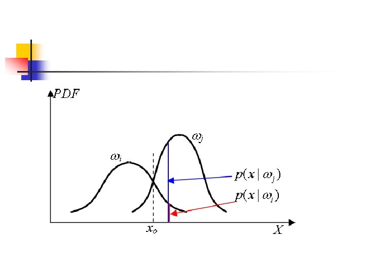
Bayes Classifier for Gaussian Distribution Consider a 1 -dimensional feature space (n = 1) and two classes (M = 2) case. The feature vector X has a normal distribution in each class. n For class i, . Thus, n

n If the two classes are equally likely to occur, i. e. , Then, the decision boundary is Xo. pdf of 2 pdf of 1 m 1 Assigning to class 1 Xo m 2 X Assigning to class 2

n n For an n-dimensional feature space and M -class case, where Ci is the covariance matrix of feature vector X for class i.

n For Gaussian distribution we usually use n Therefore,

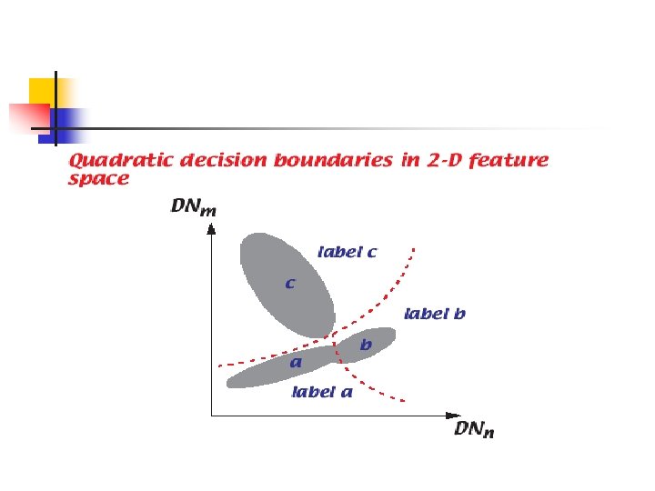
n We can also choose The above decision function is a quadratic function and therefore, the decision boundaries are quadratic curves. n If the feature vector is truly multivariate Gaussian, the Bayes classifier is the optimal classifier. n

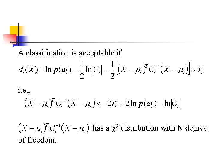
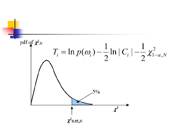
Classifier Threshold n n It is implicit in the above classification algorithms that pixels at every point in feature space will be classified into one of the available classes, irrespective of how small the actual probabilities of class membership are. Such situation can be dealt with by adopting thresholds to the decision process.

n In practice, thresholds are applied to the discriminant functions and not the probability densities, i. e. ,

n n The decision if for all A pixel will not be classified if , and.

n n If all covariance matrices are equal, Ci = C for i=1, 2, …, M, then If C = I (identity matrix) and all classes are equally likely to occur, then Decision function of the minimum distance classifier.

Assessing the Classification Accuracies n The confusion matrix (also known as the error matrix)

EO: error of omission n EC: error of commission n

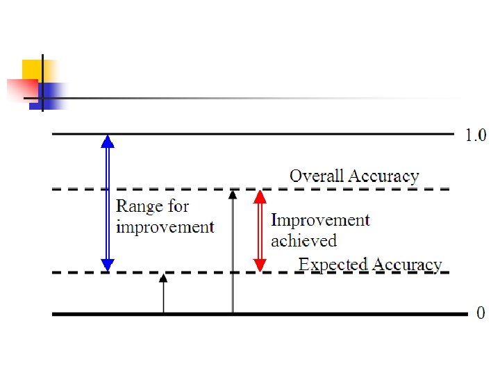
The Kappa analysis n The expected accuracy is the accuracy expected based on chance, or the expected accuracy if we randomly assign class values to each pixel.

1 overall accuracy =1 OA = error by our classification = n 1 expected accuracy =1 EA = error by random classification = n

Feature Reduction (Ch. 10, Remote Sensing Digital Image Analysis, Richards, 1995) n n n There may be many features (including spectral and textural features) available to users for image classification. Features that do not aid discrimination, by contributing little to the separability of different classes should be discarded. Removal of least effective features is referred to as feature selection, this being one form of feature reduction.

n n The other form of feature reduction is to transform the pixel vector into a new set of coordinates in which the features that can be removed are made more evident. Feature reduction is performed by checking how separable various classes remain when reduced sets of features are used. For such purpose, a measure of separability of classes is required.

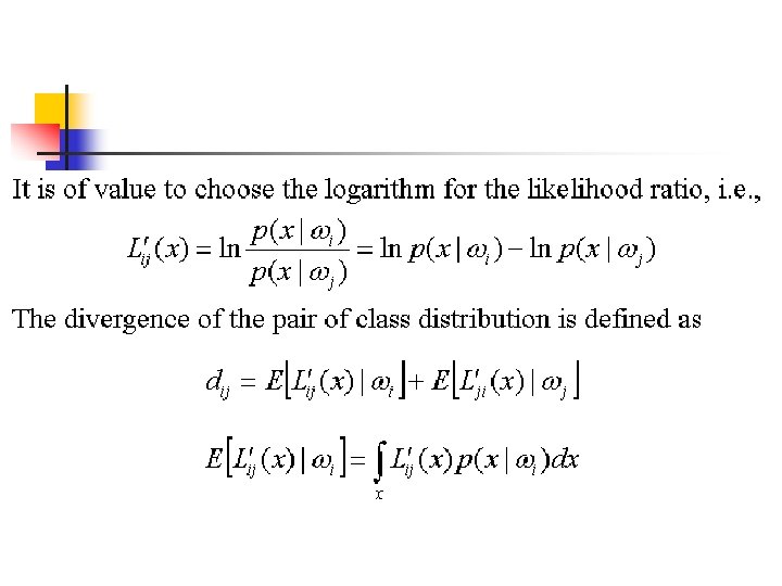
Divergence n Divergence is a measure of the separability of a pair of distributions that has its basis in their degree of overlap. It is defined in terms of the likelihood ratio where and are respectively the probability density of classes and at the position x.

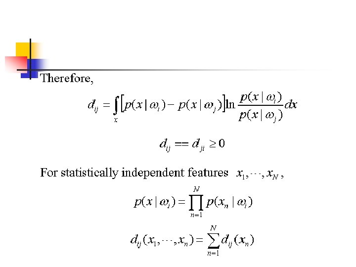
Since divergence is never negative it follows therefore that In other words, divergence never decreases as the number of features is increased.

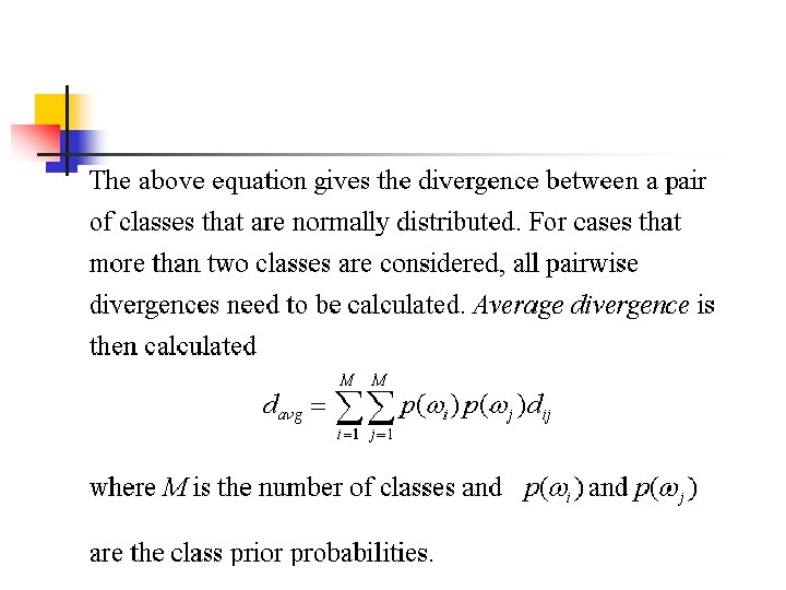
Divergence of a pair of multivariate normal distributions n Suppose that and are normal distributions with means and covariances of mi and mj and j respectively. It can be shown that