Multisource materialized views maintenance Josep Silva Jorge Belenguer

Multi-source materialized views maintenance Josep Silva, Jorge Belenguer, Matilde Celma Dpto. de Sistemas Informáticos y Computación Universidad Politécnica de Valencia. (España)

Multi-source materialized views maintenance Outline Problem statement l Goal. l Propossal. l Conclusions. l

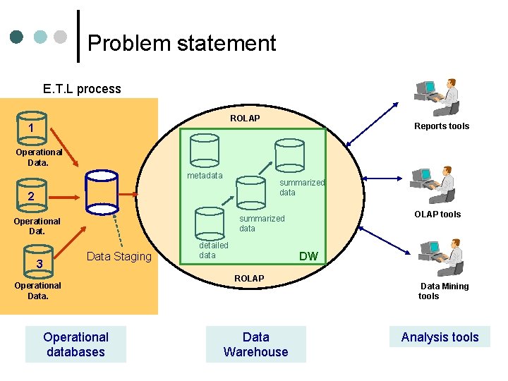
Problem statement E. T. L process ROLAP 1 Reports tools Operational Data. metadata summarized data 2 Data Staging 3 OLAP tools summarized data Operational Data. Operational databases detailed data DW ROLAP Data Warehouse Data Mining tools Analysis tools

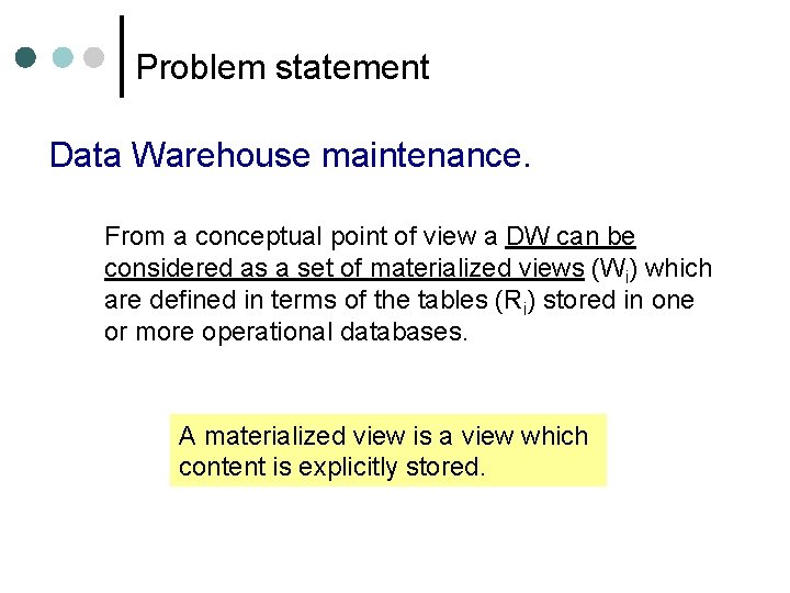
Problem statement Data Warehouse maintenance. From a conceptual point of view a DW can be considered as a set of materialized views (Wi) which are defined in terms of the tables (Ri) stored in one or more operational databases. A materialized view is a view which content is explicitly stored.

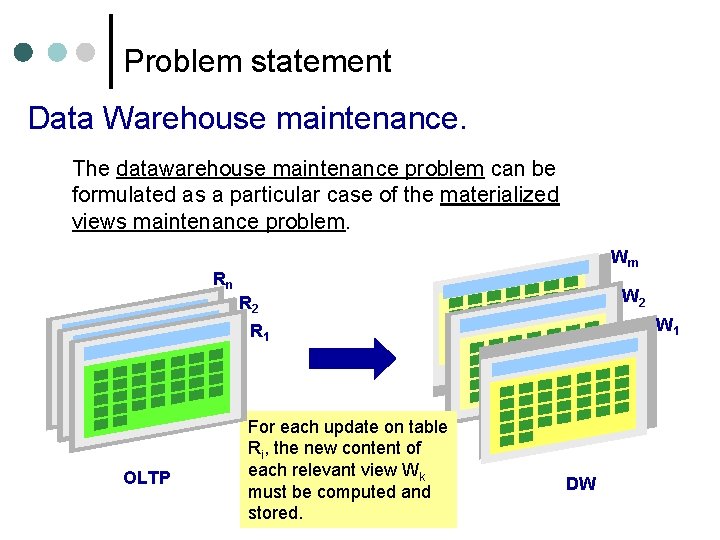
Problem statement Data Warehouse maintenance. The datawarehouse maintenance problem can be formulated as a particular case of the materialized views maintenance problem. Wm Rn W 2 R 2 W 1 R 1 OLTP For each update on table Ri, the new content of each relevant view Wk must be computed and stored. DW

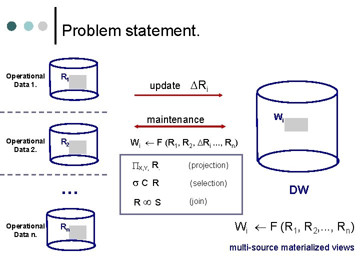
Problem statement. Operational Data 1. R 1 update Ri Wi maintenance Operational Data 2. R 2 … Operational Data n. Rn Wi F (R 1, R 2, Ri. . . , Rn) X, Y, R. (projection) C R (selection) R S (join) DW Wi F (R 1, R 2, . . . , Rn) multi-source materialized views

Goal. We proposse a solution for the multi-source materialized views maintenance problem. Characteristics of the solution: -Use of auxiliary materialized views defined over single data sources -Use of a metric which helps the designer to chosse the optimal configuration of these auxiliary views.

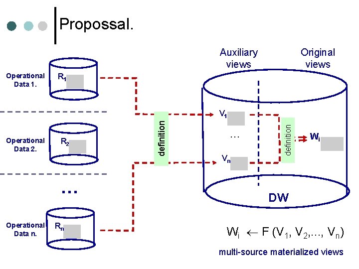
Propossal. Auxiliary views Operational Data 1. Original views R 1 R 2 … Operational Data n. Rn … Vn definition Operational Data 2. definition V 1 Wi DW Wi F (V 1, V 2, . . . , Vn) multi-source materialized views

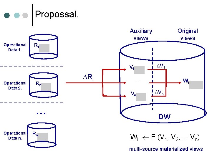
Propossal. Auxiliary views Operational Data 1. R 1 V 1 Operational Data 2. R 2 Ri … Vn … Operational Data n. Original views Rn Wi Vn DW Wi F (V 1, V 2, . . . , Vn) multi-source materialized views

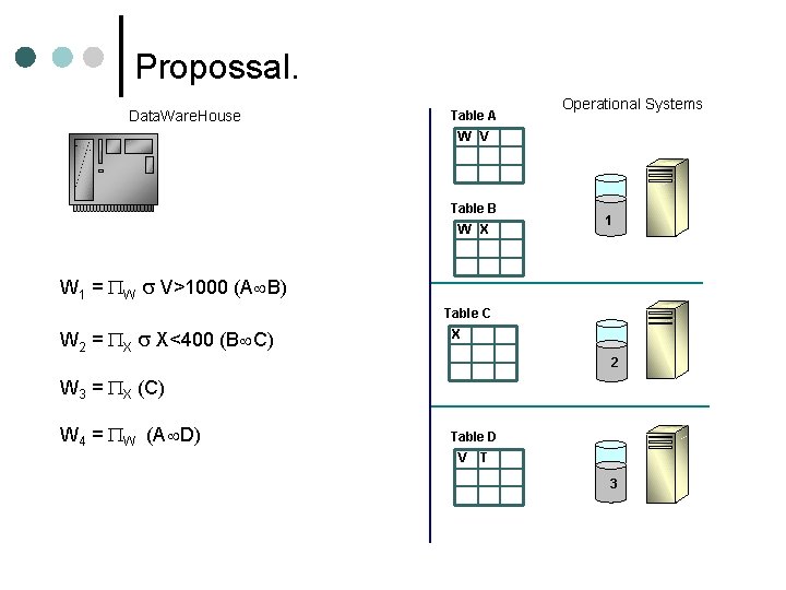
Propossal. Data. Ware. House Table A Operational Systems W V Table B W X 1 W 1 = W V>1000 (A B) Table C W 2 = X X<400 (B C) X 2 2 W 3 = X (C) W 4 = W (A D) Table D V T 3 3

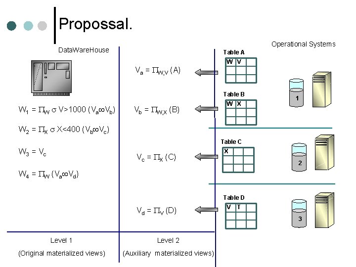
Propossal. Operational Systems Data. Ware. House Table A W V Va = W, V (A) Table B W 1 = W V>1000 (Va Vb) Vb = W, X (B) W X 1 W 2 = X X<400 (Vb Vc) Table C W 3 = Vc Vc = X (C) X 2 2 W 4 = W (Va Vd) Table D Vd = V (D) Level 1 Level 2 (Original materialized views) (Auxiliary materialized views) V T 3 3

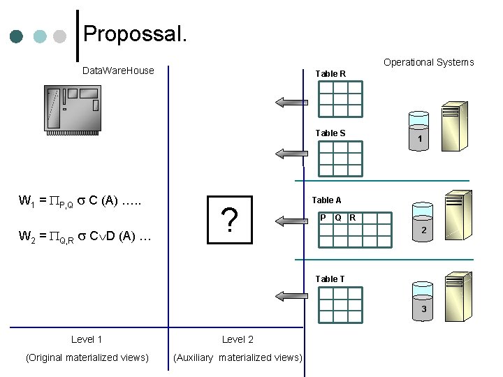
Propossal. Operational Systems Data. Ware. House Table R Table S W 1 = P, Q C (A) …. . W 2 = Q, R C D (A) … ? 1 Table A P Q R 2 2 Table T 3 3 Level 1 Level 2 (Original materialized views) (Auxiliary materialized views)

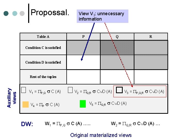
Propossal. Table A View V 3: unnecessary information P Q R Condition C is satisfied Condition D is satisfied Auxiliary views Rest of the tuples V 1 = P, Q C (A) V 4 = P C (A) DW: V 2 = Q, R C D (A) V 3 = P, Q, R C D (A) V 5 = Q, R C D (A) W 1 = P, Q C (A) …. . W 2 = Q, R C D (A) … Original materialized views

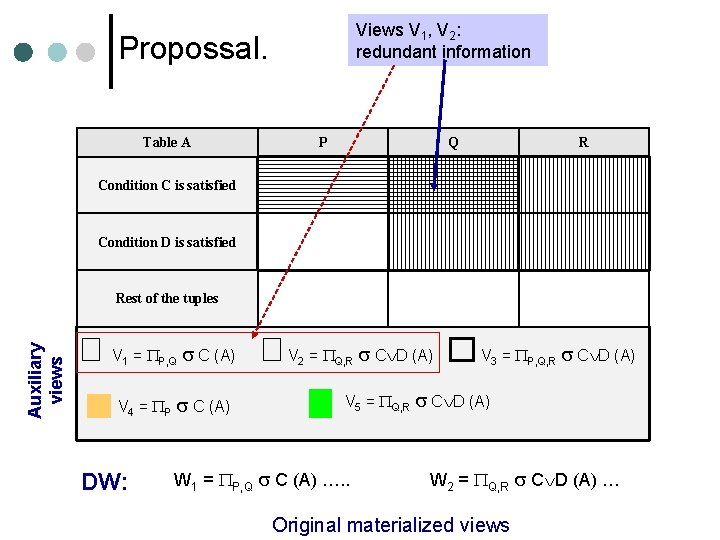
Views V 1, V 2: redundant information Propossal. Table A P Q R Condition C is satisfied Condition D is satisfied Auxiliary views Rest of the tuples V 1 = P, Q C (A) V 4 = P C (A) DW: V 2 = Q, R C D (A) V 3 = P, Q, R C D (A) V 5 = Q, R C D (A) W 1 = P, Q C (A) …. . W 2 = Q, R C D (A) … Original materialized views

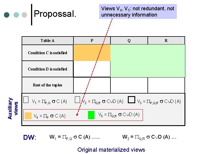
Views V 4, V 5: not redundant, not unnecessary information Propossal. Table A P Q R Condition C is satisfied Condition D is satisfied Auxiliary views Rest of the tuples V 1 = P, Q C (A) V 4 = P C (A) DW: V 2 = Q, R C D (A) V 3 = P, Q, R C D (A) V 5 = Q, R C D (A) W 1 = P, Q C (A) …. . W 2 = Q, R C D (A) … Original materialized views

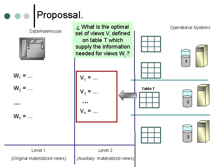
Propossal. Data. Ware. House ¿ What is the optimal set of views Vi defined on table T which supply the information needed for views Wj ? Operational Systems 1 W 1 = … W 2 = … V 1 = … Table T V 2 = … 2 2 … … Wn = … Vn = … 3 3 Level 1 Level 2 (Original materialized views) (Auxiliary materialized views)

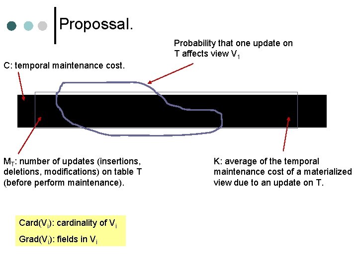
Propossal. Probability that one update on T affects view V 1 C: temporal maintenance cost. MT: number of updates (insertions, deletions, modifications) on table T (before perform maintenance). Card(Vi): cardinality of Vi Grad(Vi): fields in Vi K: average of the temporal maintenance cost of a materialized view due to an update on T.

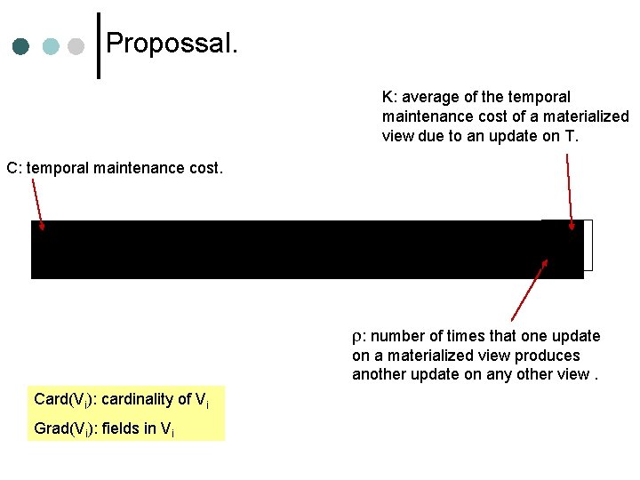
Propossal. K: average of the temporal maintenance cost of a materialized view due to an update on T. C: temporal maintenance cost. : number of times that one update on a materialized view produces another update on any other view. Card(Vi): cardinality of Vi Grad(Vi): fields in Vi

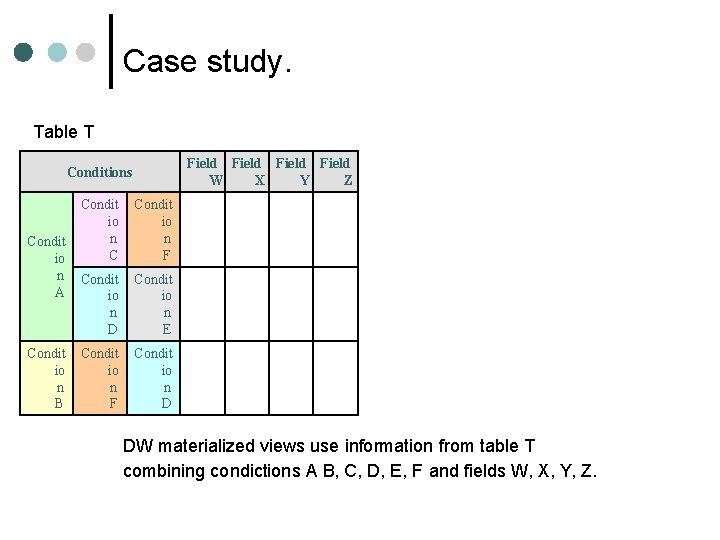
Case study. Table T Field W X Y Z Conditions Condit io n A Condit io n B Condit io n C Condit io n F Condit io n D Condit io n E Condit io n F Condit io n D DW materialized views use information from table T combining condictions A B, C, D, E, F and fields W, X, Y, Z.

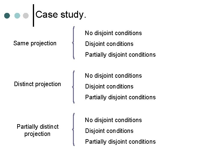
Case study. No disjoint conditions Same projection Disjoint conditions Partially disjoint conditions No disjoint conditions Distinct projection Disjoint conditions Partially disjoint conditions No disjoint conditions Partially distinct projection Disjoint conditions Partially disjoint conditions

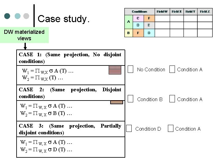
Case study. DW materialized views CASE 1: (Same projection, No disjoint conditions) W 1 = W, X A (T) … W 2 = W, X (T) … CASE 2: (Same conditions) projection, W 1 = W, X A (T) … W 2 = W, X D (T) … Condition A Condition B Condition A Disjoint W 1 = W, X A (T) … W 2 = W, X B (T) … CASE 3: (Same projection, disjoint conditions) No Condition Partially Condition D Condition A

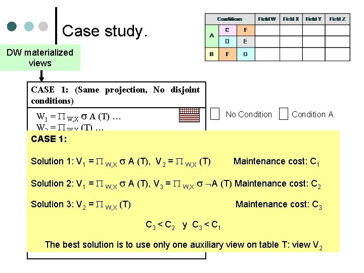
Case study. DW materialized views CASE 1: (Same projection, No disjoint conditions) No Condition A W 1 = W, X A (T) … W 2 = W, X (T) … CASE 1: CASE 2: (Same projection, Disjoint conditions) Solution 1: V 1 = W, X A (T), V 2 = W, X (T) Maintenance cost: C 1 A Condition B Condition W 1 = W, X A (T) … Solution 2: V 1 B = (T) W, X W 2 = W, … A (T), V 3 = W, X A (T) Maintenance cost: C 2 X Solution 3: 3: V(Same (T) Maintenance cost: C 3 2 = W, Xprojection, CASE Partially Condition D Condition A disjoint conditions) C 3 < C 2 y C 3 < C 1 W 1 = W, X A (T) … solution is to use only one auxiliary view on table T: view V 2 W 2 The = best W, X D (T) …

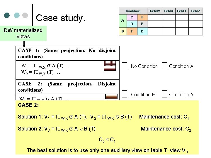
Case study. DW materialized views CASE 1: (Same projection, No disjoint conditions) W 1 = W, X A (T) … W 2 = W, X (T) … CASE 2: (Same conditions) projection, W 1 = W, X A (T) … CASE W 2 = 2: W, X B (T) … No Condition A Condition B Condition A Disjoint Solution 3: 1: V(Same A (T), V 2 Partially = W, X B (T) Maintenance cost: C 1 1 = W, Xprojection, CASE Condition D Condition A disjoint conditions) Solution 2: V 3 = W, X A B (T) Maintenance cost: C 2 W 1 = W, X A (T) … C 2 < C 1 W 2 = W, X D (T) … The best solution is to use only one auxiliary view on table T: view V 3

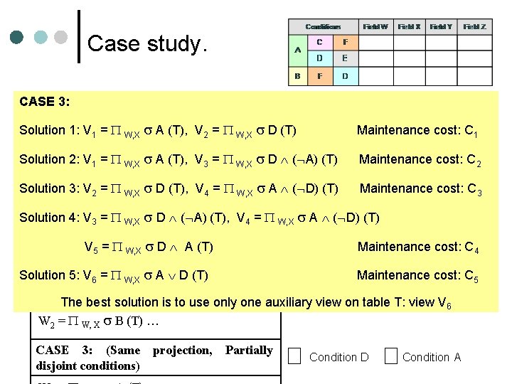
Case study. CASE 3: Solution 1: V 1 = W, X A (T), V 2 = W, X D (T) Maintenance cost: C 1 Solution 2: V 1 = W, X A (T), V 3 = W, X D ( A) (T) Maintenance cost: C 2 CASE 3: 1: V (Same projection, No disjoint Solution Maintenance cost: C 3 2 = W, X D (T), V 4 = W, X A ( D) (T) conditions) Solution ( D) (T) Condition A W =4: V 3 = AW, X (T) …D ( A) (T), V 4 = W, X ANo Condition 1 W, X W 2 = W, X (T) … V 5 = W, X D A (T) CASE 2: (Same projection, Solution 5: V 6 = W, X A D (T) conditions) Maintenance cost: C 4 Disjoint Maintenance cost: C 5 Condition B Condition A solution is to use only one auxiliary view on table T: view V 6 W 1 =The W, best X A (T) … W 2 = W, X B (T) … CASE 3: (Same projection, disjoint conditions) Partially Condition D Condition A

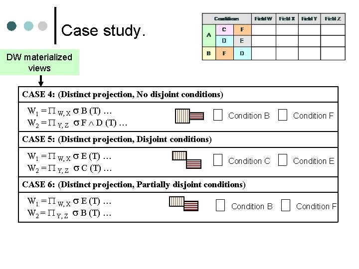
Case study. DW materialized views CASE 4: (Distinct projection, No disjoint conditions) W 1 = W, X B (T) … W 2 = Y, Z F D (T) … Condition B Condition F Condition C Condition E CASE 5: (Distinct projection, Disjoint conditions) W 1 = W, X E (T) … W 2 = Y, Z C (T) … CASE 6: (Distinct projection, Partially disjoint conditions) W 1 = W, X E (T) … W 2 = Y, Z B (T) … Condition B Condition F

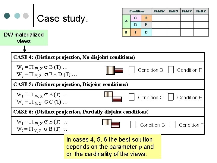
Case study. DW materialized views CASE 4: (Distinct projection, No disjoint conditions) W 1 = W, X B (T) … W 2 = Y, Z F D (T) … Condition B Condition F Condition C Condition E CASE 5: (Distinct projection, Disjoint conditions) W 1 = W, X E (T) … W 2 = Y, Z C (T) … CASE 6: (Distinct projection, Partially disjoint conditions) W 1 = W, X E (T) … W 2 = Y, Z B (T) … Condition B In cases 4, 5, 6 the best solution depends on the parameter and on the cardinality of the views. Condition F

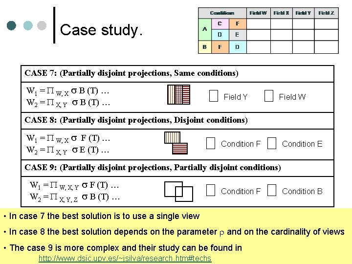
Case study. CASE 7: (Partially disjoint projections, Same conditions) W 1 = W, X B (T) … W 2 = X, Y B (T) … Field Y Field W CASE 8: (Partially disjoint projections, Disjoint conditions) W 1 = W, X F (T) … W 2 = X, Y E (T) … Condition F Condition E CASE 9: (Partially disjoint projections, Partially disjoint conditions) W 1 = W, X, Y F (T) … W 2 = X, Y, Z B (T) … Condition F Condition B • In case 7 the best solution is to use a single view • In case 8 the best solution depends on the parameter and on the cardinality of views • The case 9 is more complex and their study can be found in http: //www. dsic. upv. es/~jsilva/research. htm#techs

Conclusions In this work we have propossed a solution for the datawarehouse maintenance problem in the case of multiple data sources. Characteristics of the solution: ¢Use of auxiliary materialized views defined over single data sources ¢Use of a metric which helps the designer to chosse the optimal configuration of these auxiliary views.