Multiscale Models for Network Traffic Vinay Ribeiro Rolf

Multiscale Models for Network Traffic Vinay Ribeiro Rolf Riedi, Matt Crouse, Rich Baraniuk Dept. of Electrical Engineering Rice University (Houston, Texas)

Outline • Multiscale nature of network traffic • Wavelets • Wavelet models for traffic • Network inference applications

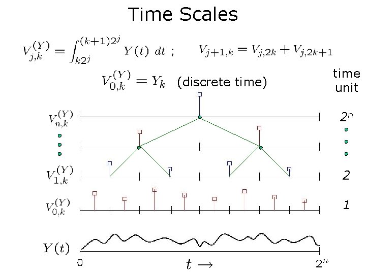
Time Scales (discrete time) time unit 2 n 2 1

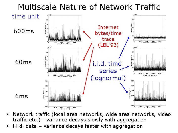
Multiscale Nature of Network Traffic time unit 600 ms 60 ms Internet bytes/time trace (LBL’ 93) i. i. d. time series (lognormal) 6 ms • Network traffic (local area networks, wide area networks, video traffic etc. ) - variance decays slowly with aggregation • i. i. d. data – variance decays faster with aggregation

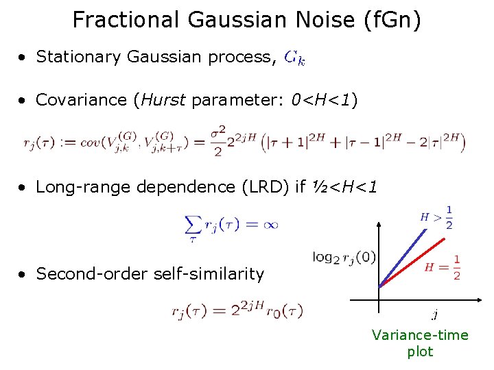
Fractional Gaussian Noise (f. Gn) • Stationary Gaussian process, • Covariance (Hurst parameter: 0<H<1) • Long-range dependence (LRD) if ½<H<1 • Second-order self-similarity Variance-time plot

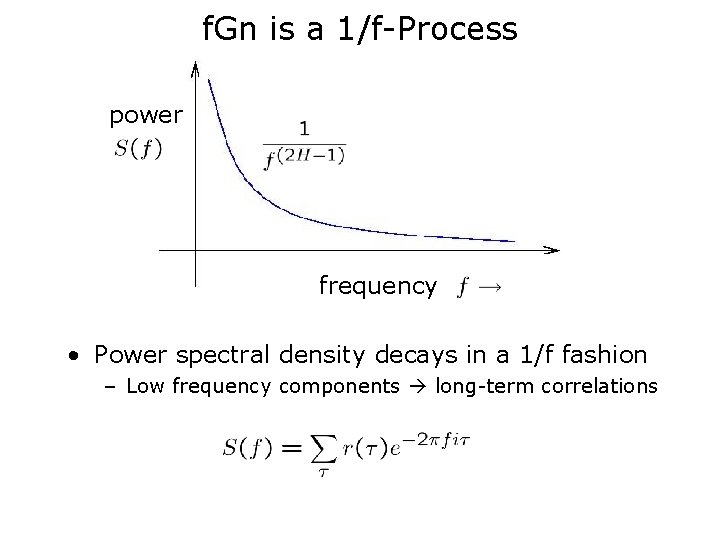
f. Gn is a 1/f-Process power frequency • Power spectral density decays in a 1/f fashion – Low frequency components long-term correlations

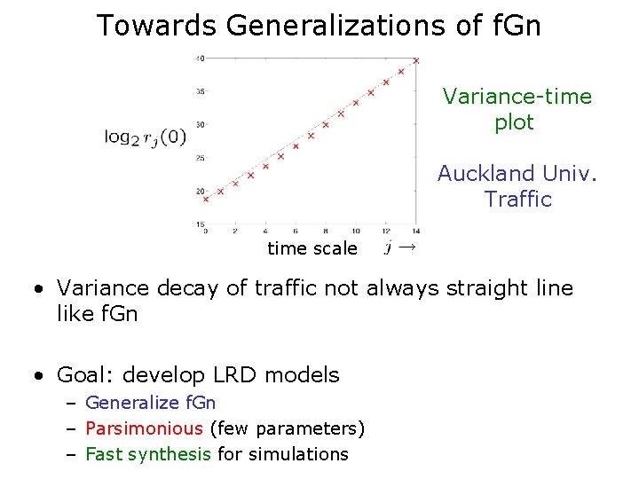
Towards Generalizations of f. Gn Variance-time plot Auckland Univ. Traffic time scale • Variance decay of traffic not always straight line like f. Gn • Goal: develop LRD models – Generalize f. Gn – Parsimonious (few parameters) – Fast synthesis for simulations

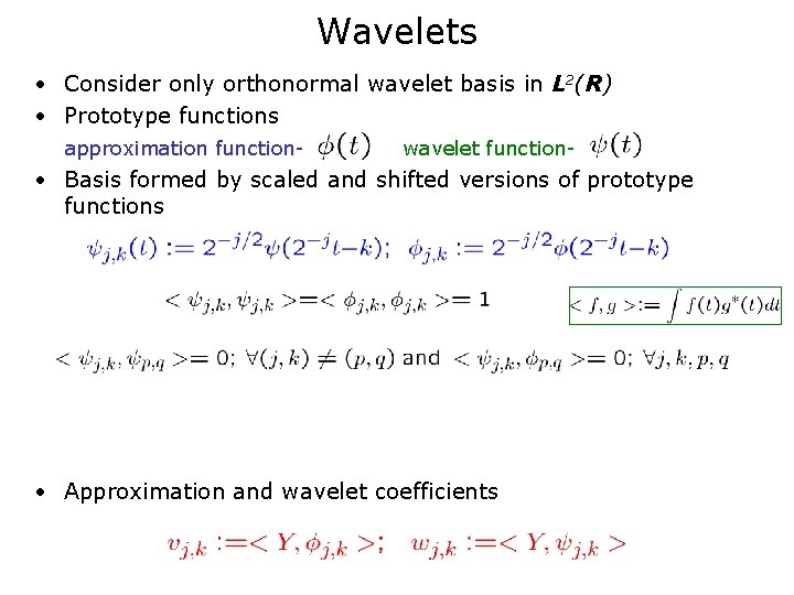
Wavelets • Consider only orthonormal wavelet basis in L 2(R) • Prototype functions approximation function- wavelet function- • Basis formed by scaled and shifted versions of prototype functions • Approximation and wavelet coefficients

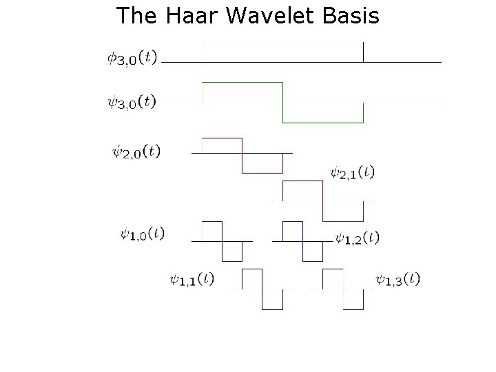
The Haar Wavelet Basis

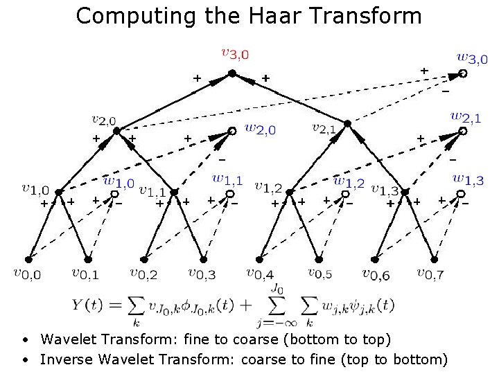
Computing the Haar Transform • Wavelet Transform: fine to coarse (bottom to top) • Inverse Wavelet Transform: coarse to fine (top to bottom)

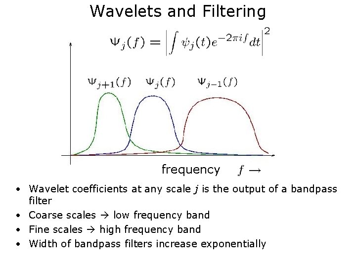
Wavelets and Filtering frequency • Wavelet coefficients at any scale j is the output of a bandpass filter • Coarse scales low frequency band • Fine scales high frequency band • Width of bandpass filters increase exponentially

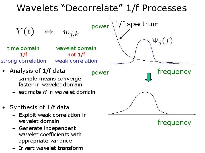
Wavelets “Decorrelate” 1/f Processes power time domain 1/f strong correlation 1/f spectrum wavelet domain not 1/f weak correlation • Analysis of 1/f data power – sample means converge faster in wavelet domain – estimate H in wavelet domain frequency • Synthesis of 1/f data – Exploit weak correlation in wavelet domain – Generate independent wavelet coefficients with appropriate variance – Invert wavelet transform frequency

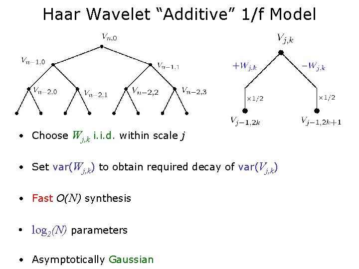
Haar Wavelet “Additive” 1/f Model • Choose Wj, k i. i. d. within scale j • Set var(Wj, k) to obtain required decay of var(Vj, k) • Fast O(N) synthesis • log 2(N) parameters • Asymptotically Gaussian

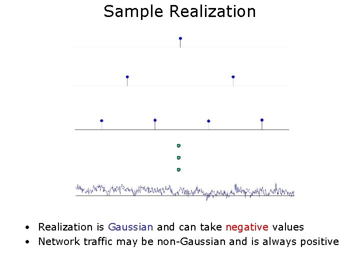
Sample Realization • Realization is Gaussian and can take negative values • Network traffic may be non-Gaussian and is always positive

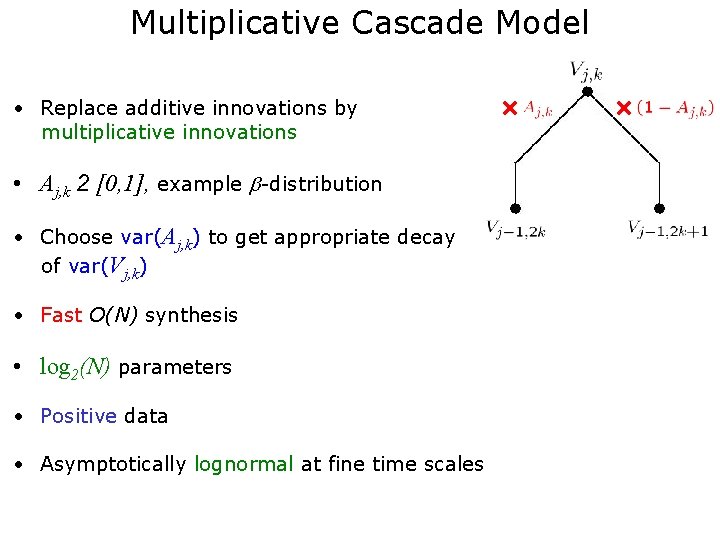
Multiplicative Cascade Model • Replace additive innovations by multiplicative innovations • Aj, k 2 [0, 1], example -distribution • Choose var(Aj, k) to get appropriate decay of var(Vj, k) • Fast O(N) synthesis • log 2(N) parameters • Positive data • Asymptotically lognormal at fine time scales

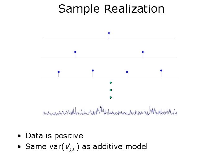
Sample Realization • Data is positive • Same var(Vj, k) as additive model

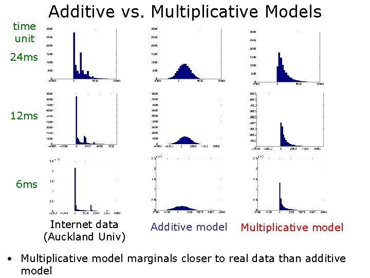
time unit Additive vs. Multiplicative Models 24 ms 12 ms 6 ms Internet data (Auckland Univ) Additive model Multiplicative model • Multiplicative model marginals closer to real data than additive model

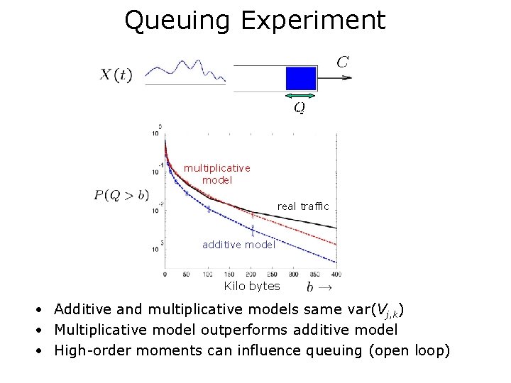
Queuing Experiment multiplicative model real traffic additive model Kilo bytes • Additive and multiplicative models same var(Vj, k) • Multiplicative model outperforms additive model • High-order moments can influence queuing (open loop)

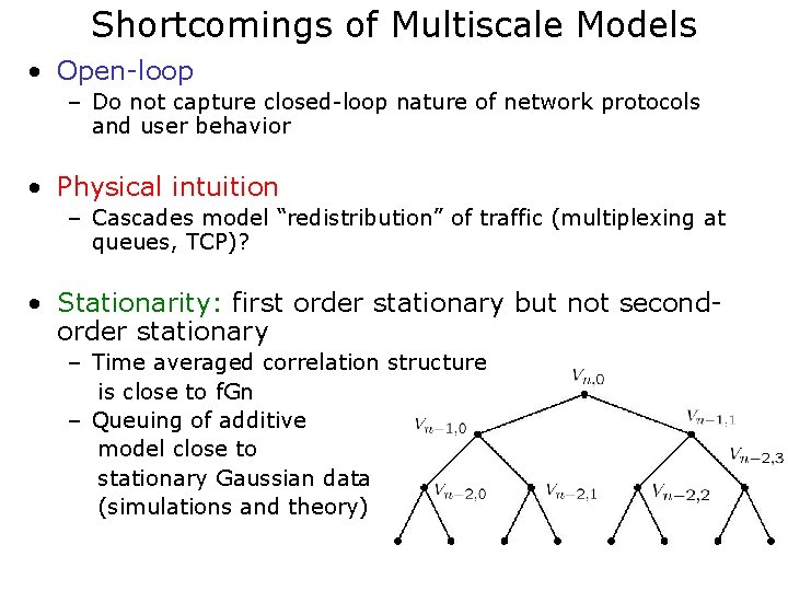
Shortcomings of Multiscale Models • Open-loop – Do not capture closed-loop nature of network protocols and user behavior • Physical intuition – Cascades model “redistribution” of traffic (multiplexing at queues, TCP)? • Stationarity: first order stationary but not secondorder stationary – Time averaged correlation structure is close to f. Gn – Queuing of additive model close to stationary Gaussian data (simulations and theory)

Selected References • Self-similar traffic and networks (upto 1996) – W. Willinger, M. Taqqu, A. Erramilli, “A bibliographical guide to self-similar traffic and performance modeling for modern high-speed networks”, Stochastic Networks: Theory and Applications, vol. 4, Oxford Univ. Press, 1996. • Wavelets – S. Burrus and R. Gopinath, “Introduction to Wavelets and Wavelet Transforms”, Prentice Hall, 1998. – I. Daubechies, “Ten lectures on wavelets”, SIAM, New York, 1992. • Additive model – S. Ma and C. Ji, “Modeling heterogeneous network traffic in wavelet domain”, IEEE Trans. Networking, vol. 9, no. 5, Oct 2001. • Multiplicative model – R. Riedi, M. Crouse, V. Ribeiro, R. Baraniuk, “A multifractal wavelet model with application to network traffic”, IEEE Trans. Info. Theory, vol. 45, no. 3, April 1999. – A. Feldmann, A. C. Gilbert, W. Willinger, “Data networks as cascasdes: investigating the multifractal nature of Internet WAN traffic”, ACM SIGCOMM, pp. 42 -55, 1998. – P. Mannersalo and I. Norros, “Multifractal analysis of real ATM traffic: A first look”, Technical report, VTT Information Technology, 1997, COST 257 TD(97)19,

Network Inference Applications

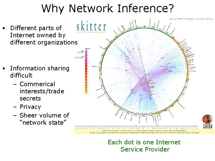
Why Network Inference? • Different parts of Internet owned by different organizations • Information sharing difficult – Commerical interests/trade secrets – Privacy – Sheer volume of “network state” Each dot is one Internet Service Provider

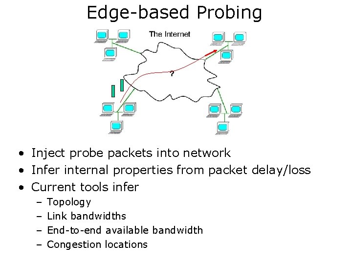
Edge-based Probing • Inject probe packets into network • Infer internal properties from packet delay/loss • Current tools infer – – Topology Link bandwidths End-to-end available bandwidth Congestion locations

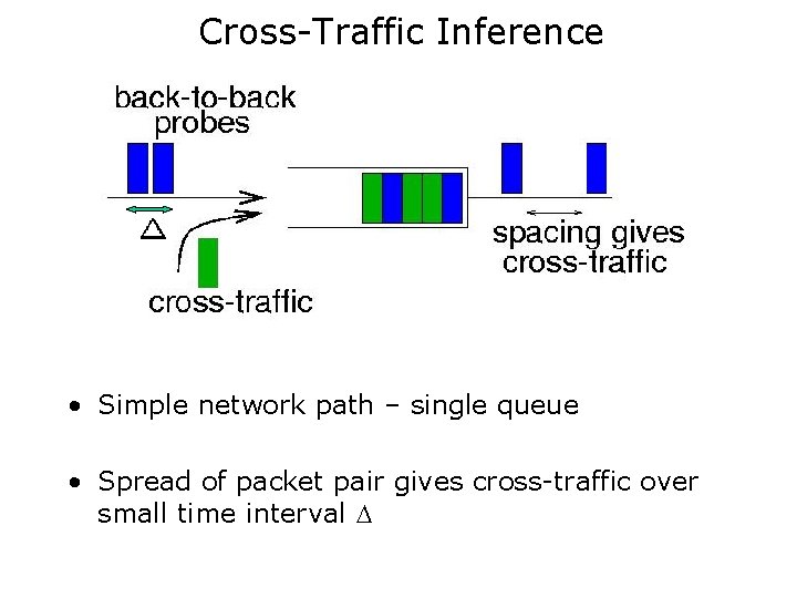
Cross-Traffic Inference • Simple network path – single queue • Spread of packet pair gives cross-traffic over small time interval

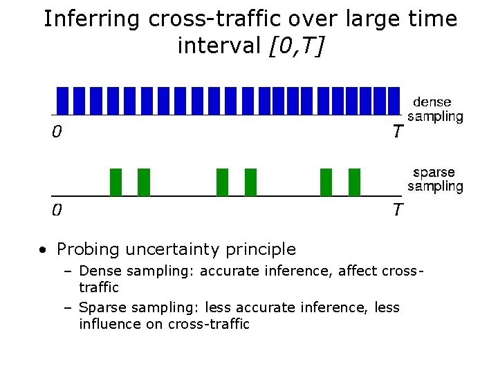
Inferring cross-traffic over large time interval [0, T] • Probing uncertainty principle – Dense sampling: accurate inference, affect crosstraffic – Sparse sampling: less accurate inference, less influence on cross-traffic

Problem Statement Given N probe pairs, how must we space them over time interval [0, T] to optimally estimate the total cross-traffic in [0, T] • Answer depends on – cross-traffic – optimality criterion

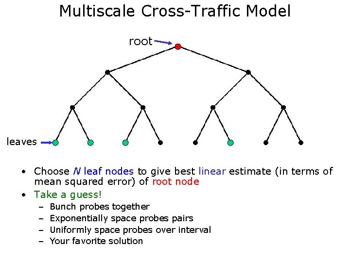
Multiscale Cross-Traffic Model root leaves • Choose N leaf nodes to give best linear estimate (in terms of mean squared error) of root node • Take a guess! – – Bunch probes together Exponentially space probes pairs Uniformly space probes over interval Your favorite solution

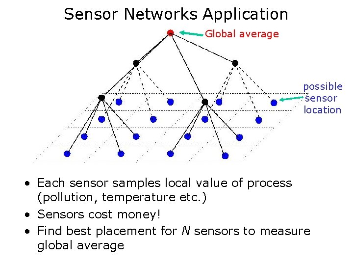
Sensor Networks Application Global average possible sensor location • Each sensor samples local value of process (pollution, temperature etc. ) • Sensors cost money! • Find best placement for N sensors to measure global average

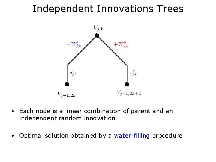
Independent Innovations Trees • Each node is a linear combination of parent and an independent random innovation • Optimal solution obtained by a water-filling procedure

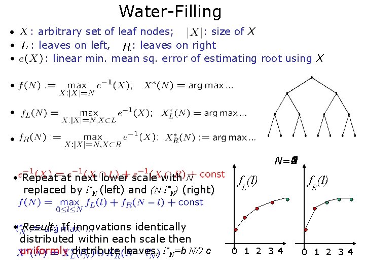
Water-Filling • • • : arbitrary set of leaf nodes; : size of X : leaves on left, : leaves on right : linear min. mean sq. error of estimating root using X • • • 3 4 2 1 N=0 • Repeat at next lower scale with N replaced by l*N (left) and (N-l*N) (right) • Result: If innovations identically distributed within each scale then uniformly distribute leaves, l*N=b N/2 c f (l) L 0 1 2 34 f (l) R 0 1 2 34

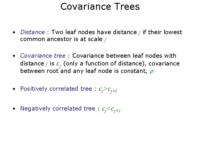
Covariance Trees • Distance : Two leaf nodes have distance j if their lowest common ancestor is at scale j • Covariance tree : Covariance between leaf nodes with distance j is cj (only a function of distance), covariance between root and any leaf node is constant, • Positively correlated tree : cj>cj+1 • Negatively correlated tree : cj<cj+1

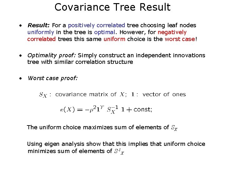
Covariance Tree Result • Result: For a positively correlated tree choosing leaf nodes uniformly in the tree is optimal. However, for negatively correlated trees this same uniform choice is the worst case! • Optimality proof: Simply construct an independent innovations tree with similar correlation structure • Worst case proof: The uniform choice maximizes sum of elements of SX Using eigen analysis show that this implies that uniform choice minimizes sum of elements of S-1 X

Future Directions • Sampling – More general tree structures – Non-linear estimates – Non-tree stochastic processes • Traffic estimation – More complex networks • Sensor networks – jointly optimize with other constraints like power transmission

References • Estimation on multiscale trees – A. Willsky, “Multiresolution Markov models for signal and image processing”, Proc. of the IEEE 90(8), August 2002. • Optimal sampling on trees – V. Ribeiro, R. Riedi, and R. Baraniuk, “Optimal sampling strategies for multiscale models and their application to computer networks”, preprint.