Multiplicative Interaction Models Thomas Brambor William Roberts Clark

Multiplicative Interaction Models Thomas Brambor, William Roberts Clark, Matt Golder • use multiplicative interaction models whenever the hypothesis to test is conditional • include all constitutive terms in interaction model specifications • Do not interpret constitutive terms as if they are unconditional marginal effects • calculate substantively meaningful marginal effects and standard errors

Variance • the variance is the expected value of the squared difference between the variable's realization and the variable's mean • covariance is a measure of how much two random variables change together

Variance of Interaction Models

X 2 is also an interaction term. It means that the effect of X is conditioned on X

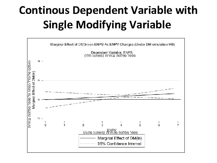
Continous Dependent Variable with Single Modifying Variable – STATA code * ******************************** *; * Estimate Model: Y = b 0 + b 1 X + b 2 Z + b 3 XZ + b 4 Controls + epsilon *; * ******************************** *; regress Y X Z XZ Controls; This indicates that you will be calculating the marginal effect of X across the generate MV=(( n-1)/10); modifying range of MV (or Z) in increments of 0. 1. You may want to calculate the marginal effect of X for different increments in MV (or Z). To do this simply divide ( n 1) by a number different than 10. For example, you can divide by 100 to calculate the marginal effect of X across MV as MV increases in increments of 0. 01. replace MV=. if n >60; * ******************************** *; * Grab elements of the coefficient and variance-covariance matrix *; * that are required to calculate the marginal effect and standard errors. *; * ******************************** *; matrix b=e(b); matrix V=e(V); scalar b 1=b[1, 1]; scalar b 2=b[1, 2]; scalar b 3=b[1, 3]; scalar varb 1=V[1, 1]; scalar varb 2=V[2, 2]; scalar varb 3=V[3, 3]; scalar covb 1 b 3=V[1, 3]; scalar covb 2 b 3=V[2, 3];

* ******************************** *; * Calculate the marginal effect of X on Y for all MV values of *; * the modifying variable Z. *; * ******************************** *; This line calculates the marginal effect (or conditional beta) of X for all values of the modifying gen conb=b 1+b 3*MV if n < 60; variable MV so long as MV is less than 6. So, now we have the marginal effect of X for when MV=0, when MV=0. 1, when MV=0. 2. . . , when MV=5. 9. * ******************************** *; * Calculate the standard errors for the marginal effect of X on Y *; * for all MV values of the modifying variable Z. *; * ******************************** *; gen conse=sqrt(varb 1+varb 3*(MV 2)+2*covb 1 b 3*MV) if n < 60; * ******************************** *; * Generate upper and lower bounds of the confidence interval. *; * Specify the significance of the confidence interval. *; * ******************************** *; gen a=1. 96*conse; gen upper=conb+a; gen lower=conb-a;

* ******************************** *; * Graph the marginal effect of X on Y across the desired range of *; * the modifying variable Z. Show the confidence interval. *; * ******************************** *; graph twoway line conb MV, clwidth(medium) clcolor(blue) clcolor(black) || line upper MV, clpattern(dash) clwidth(thin) clcolor(black) || line lower MV, clpattern(dash) clwidth(thin) clcolor(black), xlabel(0 1 2 3 4 5 6, labsize(2. 5)) ylabel(-4 -2 0 2 4, labsize(2. 5)) yscale(noline) xscale(noline) legend(col(1) order(1 2) label(1 “Marginal Effect of X”) label(2 “ 95% Confidence Interval”) label(3 “ ”)) yline(0, lcolor(black)) title(“Marginal Effect of X on Y As Z Changes”, size(4)) subtitle(“ ” “Dependent Variable: Y” “ ”, size(3)) xtitle( Z, size(3) ) xsca(titlegap(2)) ytitle(“Marginal Effect of X”, size(3)) scheme(s 2 mono) graphregion(fcolor(white)); graph export h: figure 1. eps, replace;

Continous dependent variable with Two Modifying Variables Limited dependent variable with Single Modifying Variable

Source: Multiplicative Interaction Models – Thomas Brambor, William Roberts Clark, Matt Golder https: //files. nyu. edu/mrg 217/public/interaction. html