MultipleSource Shortest Paths in Planar Graphs Allowing Negative

Multiple-Source Shortest Paths in Planar Graphs Allowing Negative Lengths Philip Klein Brown University

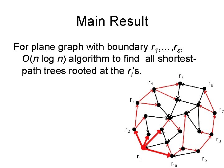
Main Result For plane graph with boundary r 1, …, rs, O(n log n) algorithm to find all shortestpath trees rooted at the ri’s.

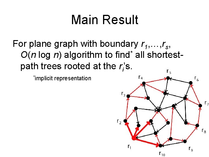
Main Result For plane graph with boundary r 1, …, rs, O(n log n) algorithm to find* all shortestpath trees rooted at the ri’s. *implicit representation

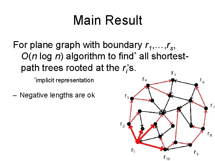
Main Result For plane graph with boundary r 1, …, rs, O(n log n) algorithm to find* all shortestpath trees rooted at the ri’s. *implicit representation – Negative lengths are ok

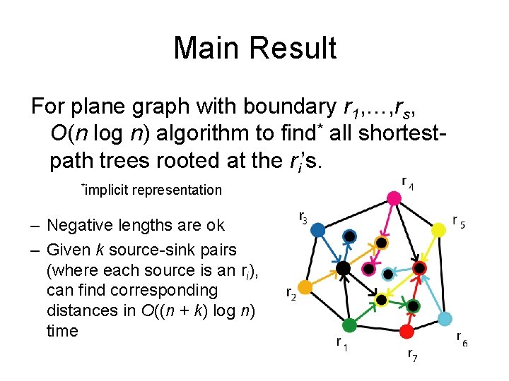
Main Result For plane graph with boundary r 1, …, rs, O(n log n) algorithm to find* all shortestpath trees rooted at the ri’s. *implicit representation – Negative lengths are ok – Given k source-sink pairs (where each source is an ri), can find corresponding distances in O((n + k) log n) time

Some Applications • Single-source shortest-path tree in planar graph with some negative lengths: O(n log n). Previous bound: O(n log 3 n) [Fakcharoenphol, Rao] – Testing feasibility of planar flow with multiple sources and sinks, and upper and lower capacities: O(n log n). – Finding a minimum ratio cut in a planar graph (used in, e. g. , segmentation of images [Cox, Rao, Zhong]): O(n log CW) where C = sum of costs, W = sum of weights.

Some Applications • Preprocessing a planar graph to admit O*( exact distance queries: O(n log 2 n). Previous bound [Fakch. , Rao]: O(n log 3 n) )-time • Preprocessing undirected planar graph to admit O(ε -1)-time approx. distance queries: O(ε-1 n log 2 n). Previous bound [Thorup]: O(ε-2 n log 3 n) (similar improvement for directed graphs) • Slightly faster dynamic algorithms for planar-graph distances (improving on [Fakch. , Rao])

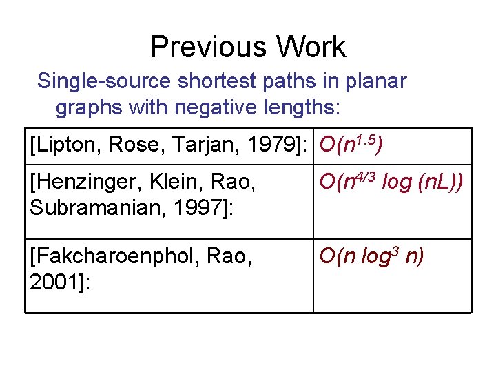
Previous Work Single-source shortest paths in planar graphs with negative lengths: [Lipton, Rose, Tarjan, 1979]: O(n 1. 5) [Henzinger, Klein, Rao, Subramanian, 1997]: O(n 4/3 log (n. L)) [Fakcharoenphol, Rao, 2001]: O(n log 3 n)

Previous Work Multiple-source shortest paths in planar graphs: [Schmidt, 1995]: For special case of n-node grid DAG, after O(n log n) preprocessing, can find distance from any node in column 0 to any other node in O(log n) time.

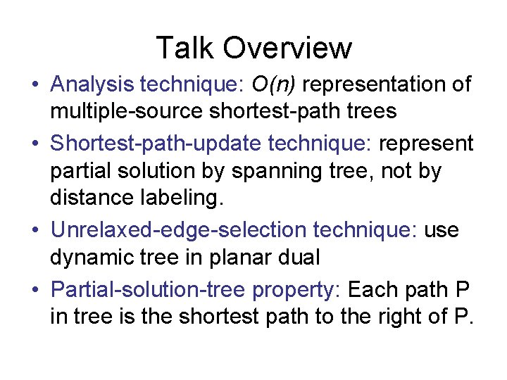
Talk Overview • Analysis technique: O(n) representation of multiple-source shortest-path trees • Shortest-path-update technique: represent partial solution by spanning tree, not by distance labeling. • Unrelaxed-edge-selection technique: use dynamic tree in planar dual • Partial-solution-tree property: Each path P in tree is the shortest path to the right of P.

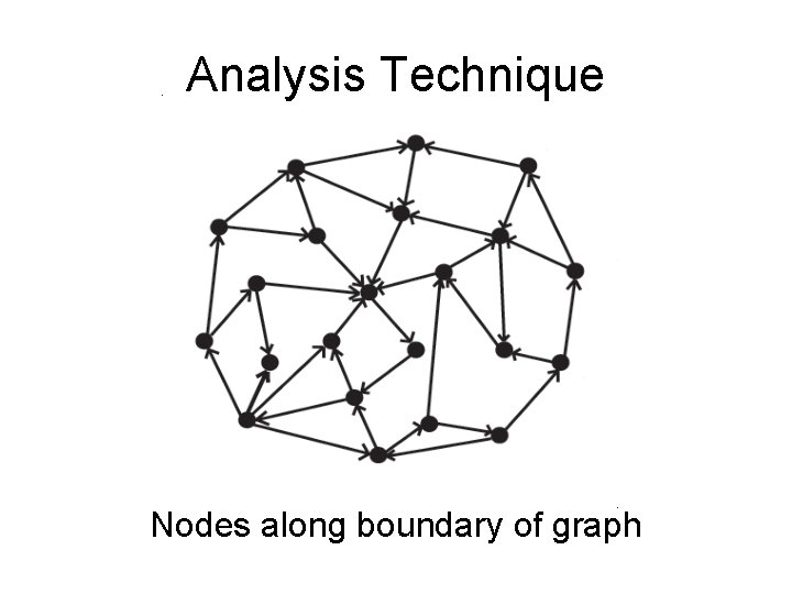
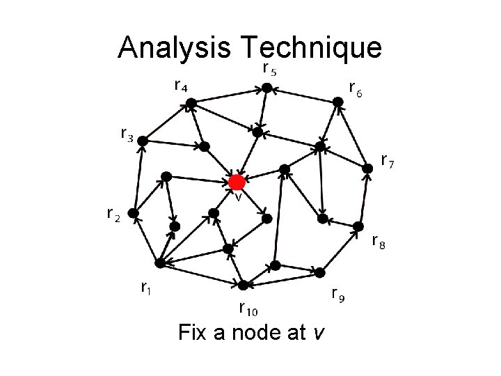
Analysis Technique Nodes along boundary of graph

Analysis Technique Fix a node at v

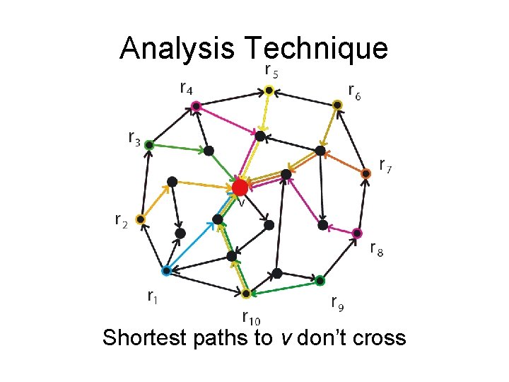
Analysis Technique Shortest paths to v don’t cross

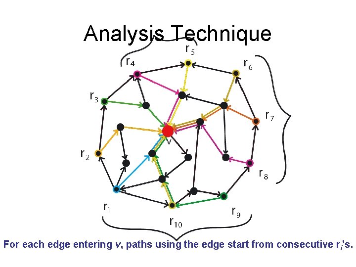
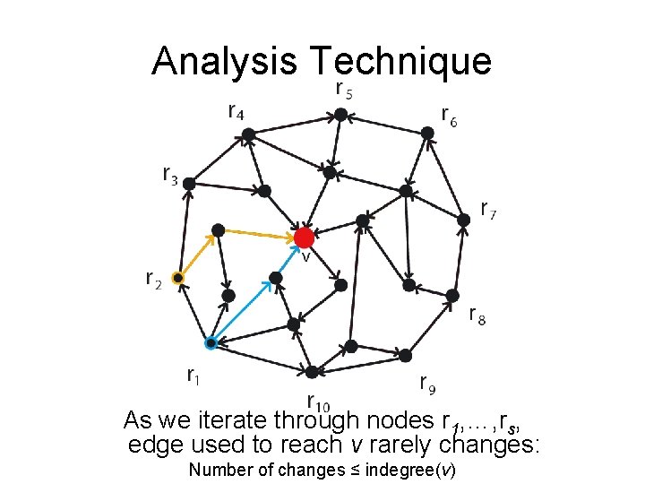
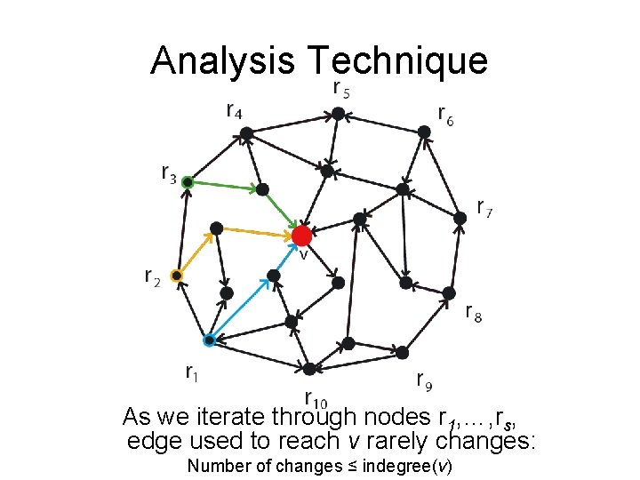
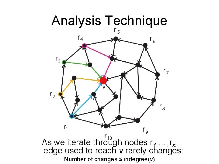
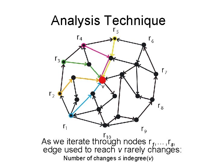
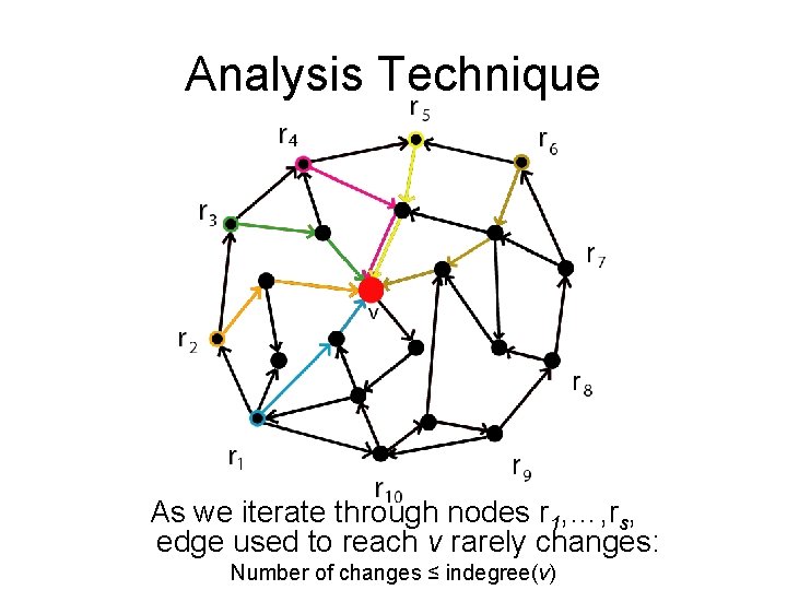
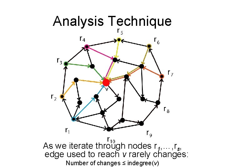
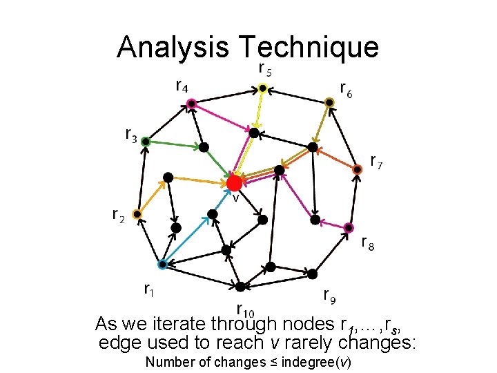
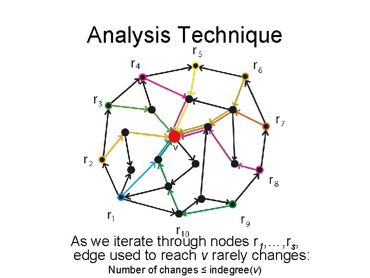
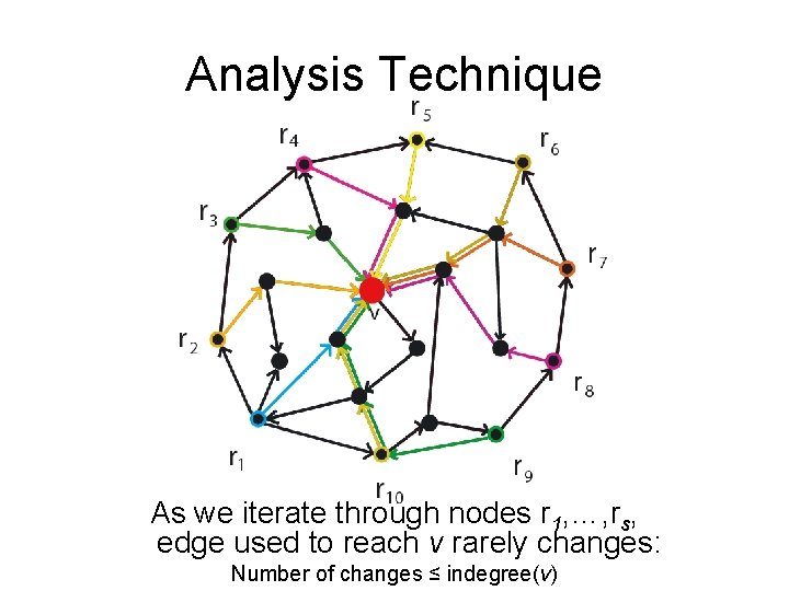
Analysis Technique For each edge entering v, paths using the edge start from consecutive ri’s.

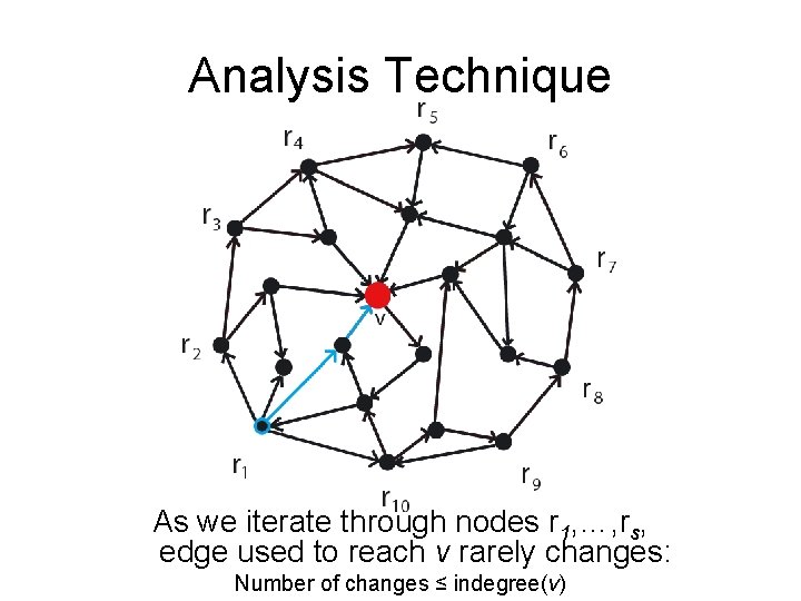
Analysis Technique As we iterate through nodes r 1, …, rs, edge used to reach v rarely changes: Number of changes ≤ indegree(v)

Analysis Technique As we iterate through nodes r 1, …, rs, edge used to reach v rarely changes: Number of changes ≤ indegree(v)

Analysis Technique As we iterate through nodes r 1, …, rs, edge used to reach v rarely changes: Number of changes ≤ indegree(v)

Analysis Technique As we iterate through nodes r 1, …, rs, edge used to reach v rarely changes: Number of changes ≤ indegree(v)

Analysis Technique As we iterate through nodes r 1, …, rs, edge used to reach v rarely changes: Number of changes ≤ indegree(v)

Analysis Technique As we iterate through nodes r 1, …, rs, edge used to reach v rarely changes: Number of changes ≤ indegree(v)

Analysis Technique As we iterate through nodes r 1, …, rs, edge used to reach v rarely changes: Number of changes ≤ indegree(v)

Analysis Technique As we iterate through nodes r 1, …, rs, edge used to reach v rarely changes: Number of changes ≤ indegree(v)

Analysis Technique As we iterate through nodes r 1, …, rs, edge used to reach v rarely changes: Number of changes ≤ indegree(v)

Analysis Technique As we iterate through nodes r 1, …, rs, edge used to reach v rarely changes: Number of changes ≤ indegree(v)

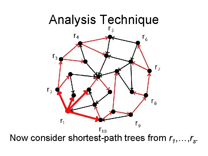
Analysis Technique Now consider shortest-path trees from r 1, …, rs.

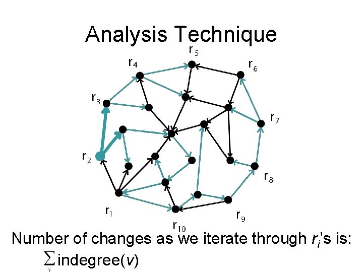
Analysis Technique Number of changes as we iterate through ri’s is: indegree(v)

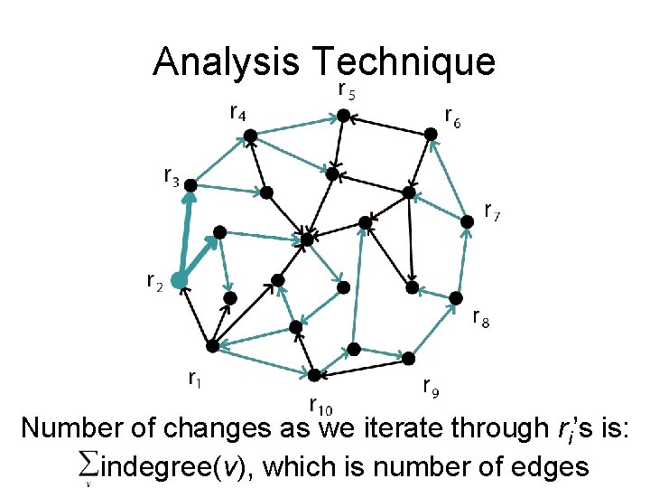
Analysis Technique Number of changes as we iterate through ri’s is: indegree(v), which is number of edges

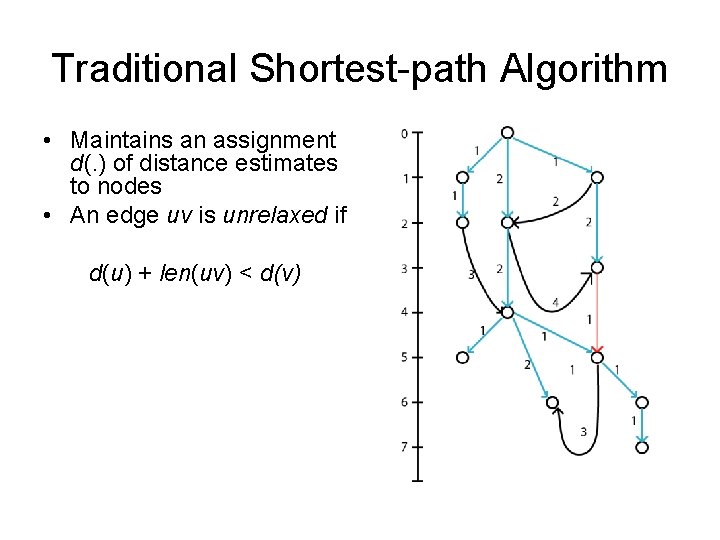
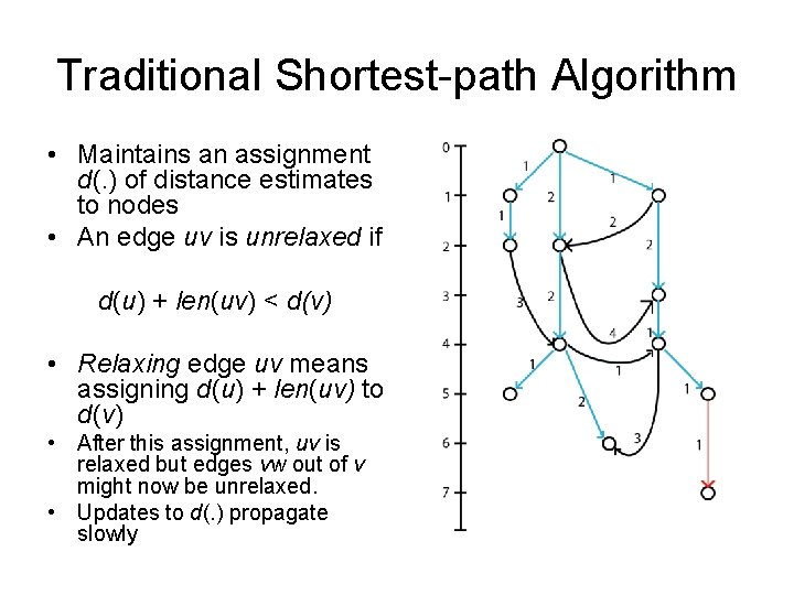
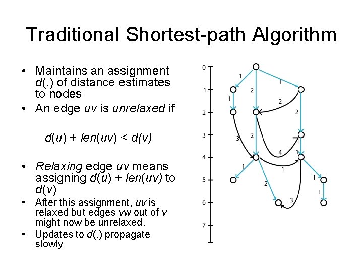
Traditional Shortest-path Algorithm • Maintains an assignment d(. ) of distance estimates to nodes • An edge uv is unrelaxed if d(u) + len(uv) < d(v)

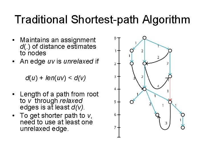
Traditional Shortest-path Algorithm • Maintains an assignment d(. ) of distance estimates to nodes • An edge uv is unrelaxed if d(u) + len(uv) < d(v) • Length of a path from root to v through relaxed edges is at least d(v). • To get shorter path to v, need to use at least one unrelaxed edge.

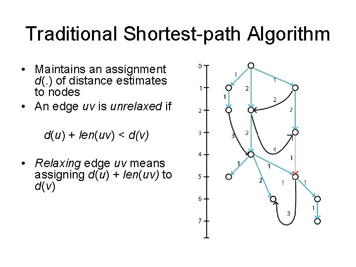
Traditional Shortest-path Algorithm • Maintains an assignment d(. ) of distance estimates to nodes • An edge uv is unrelaxed if d(u) + len(uv) < d(v) • Relaxing edge uv means assigning d(u) + len(uv) to d(v)

Traditional Shortest-path Algorithm • Maintains an assignment d(. ) of distance estimates to nodes • An edge uv is unrelaxed if d(u) + len(uv) < d(v) • Relaxing edge uv means assigning d(u) + len(uv) to d(v)

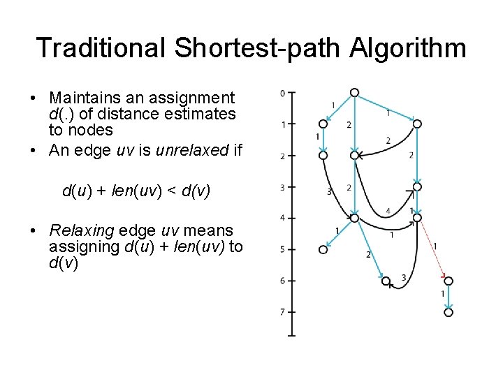
Traditional Shortest-path Algorithm • Maintains an assignment d(. ) of distance estimates to nodes • An edge uv is unrelaxed if d(u) + len(uv) < d(v) • Relaxing edge uv means assigning d(u) + len(uv) to d(v) • After this assignment, uv is relaxed but edges vw out of v might now be unrelaxed. • Updates to d(. ) propagate slowly

Traditional Shortest-path Algorithm • Maintains an assignment d(. ) of distance estimates to nodes • An edge uv is unrelaxed if d(u) + len(uv) < d(v) • Relaxing edge uv means assigning d(u) + len(uv) to d(v) • After this assignment, uv is relaxed but edges vw out of v might now be unrelaxed. • Updates to d(. ) propagate slowly

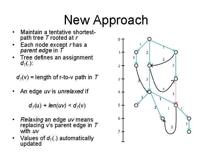
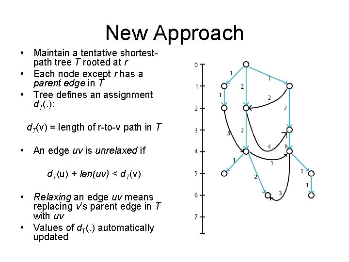
New Approach • Maintain a tentative shortestpath tree T rooted at r • Each node except r has a parent edge in T • Tree defines an assignment d. T(. ): d. T(v) = length of r-to-v path in T • An edge uv is unrelaxed if d. T(u) + len(uv) < d. T(v) • Relaxing an edge uv means replacing v’s parent edge in T with uv • Values of d. T(. ) automatically updated

New Approach • Maintain a tentative shortestpath tree T rooted at r • Each node except r has a parent edge in T • Tree defines an assignment d. T(. ): d. T(v) = length of r-to-v path in T • An edge uv is unrelaxed if d. T(u) + len(uv) < d. T(v) • Relaxing an edge uv means replacing v’s parent edge in T with uv • Values of d. T(. ) automatically updated

Generic Single-Source Algorithm • Start with some tree rooted at r. • Repeat select an unrelaxed edge relax it Until none exist • Questions: – Which tree to start with? – How to find an unrelaxed edge? – How much time is required?

Generic Single-Source Algorithm • Start with some tree rooted at r. • Repeat select an unrelaxed edge relax it Until none exist • Questions: – Which tree to start with? – How to select an unrelaxed edge? – How much time is required?

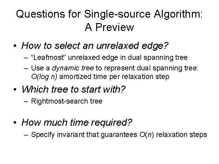
Questions for Single-source Algorithm: A Preview • How to select an unrelaxed edge? – “Leafmost” unrelaxed edge in dual spanning tree – Use a dynamic tree to represent dual spanning tree: O(log n) amortized time per relaxation step • Which tree to start with? – Rightmost-search tree • How much time required? – Specify invariant that guarantees O(n) relaxation steps

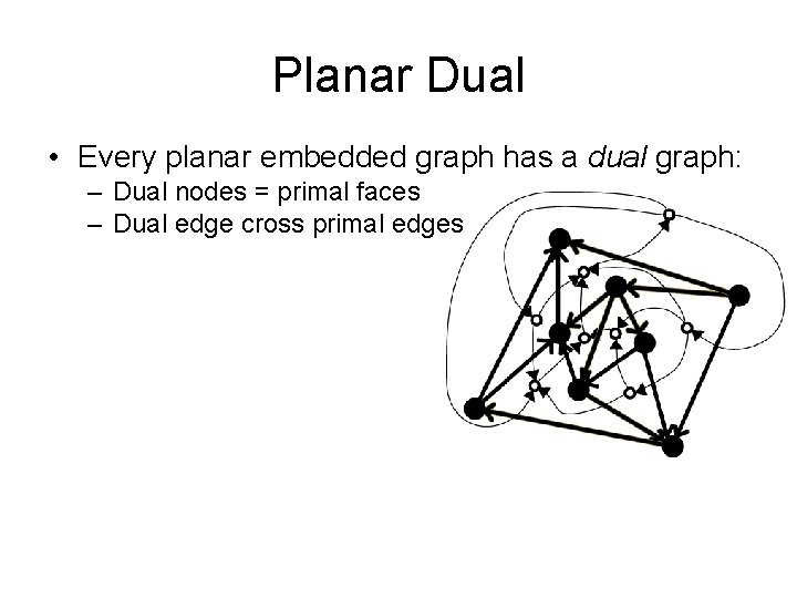
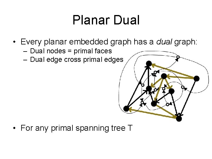
Planar Dual • Every planar embedded graph has a dual graph: – Dual nodes = primal faces – Dual edge cross primal edges

Planar Dual • Every planar embedded graph has a dual graph: – Dual nodes = primal faces – Dual edge cross primal edges • For any primal spanning tree T

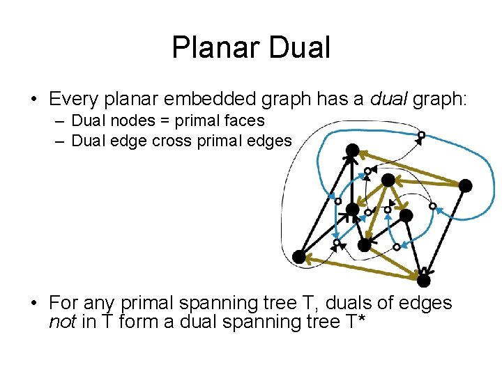
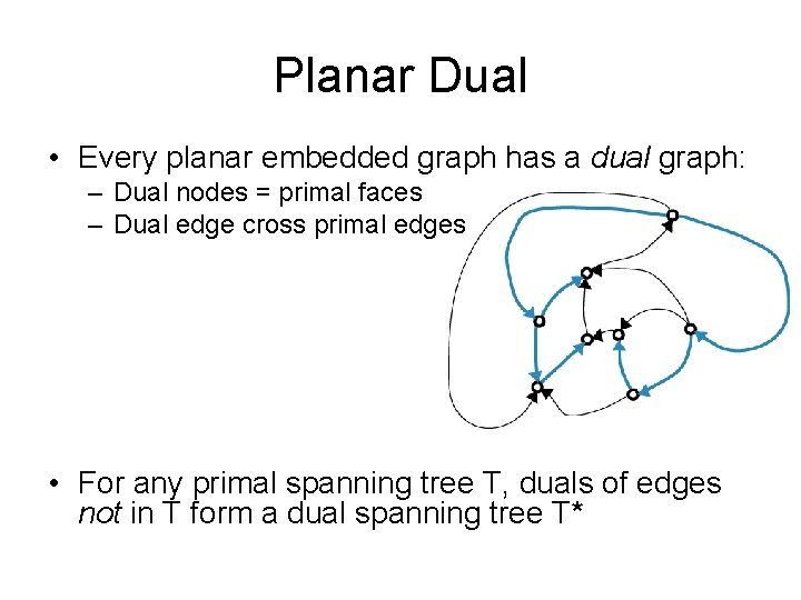
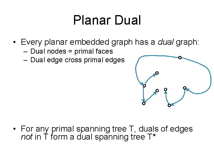
Planar Dual • Every planar embedded graph has a dual graph: – Dual nodes = primal faces – Dual edge cross primal edges • For any primal spanning tree T, duals of edges not in T form a dual spanning tree T*

Planar Dual • Every planar embedded graph has a dual graph: – Dual nodes = primal faces – Dual edge cross primal edges • For any primal spanning tree T, duals of edges not in T form a dual spanning tree T*

Planar Dual • Every planar embedded graph has a dual graph: – Dual nodes = primal faces – Dual edge cross primal edges • For any primal spanning tree T, duals of edges not in T form a dual spanning tree T*

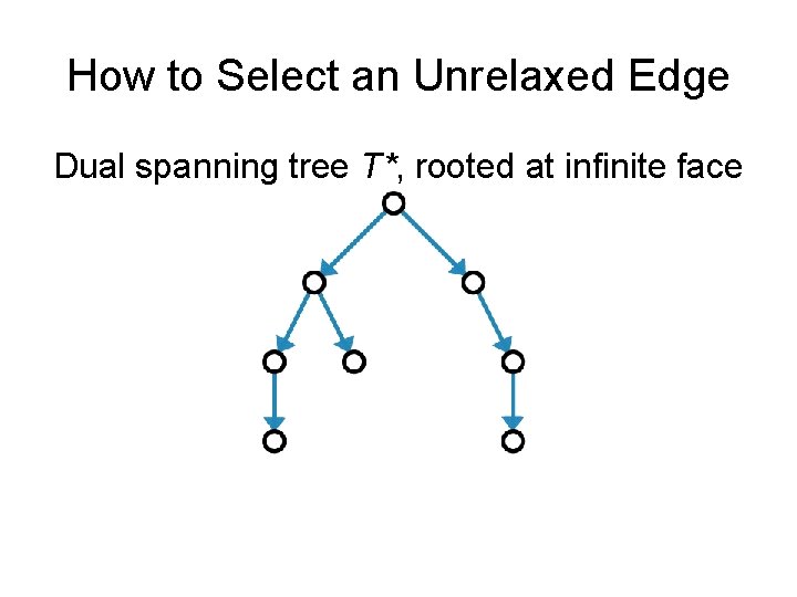
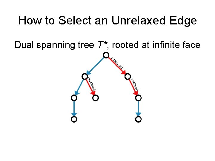
How to Select an Unrelaxed Edge Dual spanning tree T*, rooted at infinite face

How to Select an Unrelaxed Edge Dual spanning tree T*, rooted at infinite face

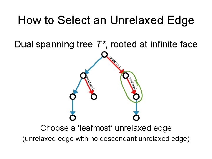
How to Select an Unrelaxed Edge Dual spanning tree T*, rooted at infinite face Choose a ‘leafmost’ unrelaxed edge (unrelaxed edge with no descendant unrelaxed edge)

Choosing Unrelaxed Edge: Implementation Use a dynamic tree data structure [Sleator, Tarjan] to represent the dual tree T*. O(log n) time per operation Structure Operations: – Cut an edge, breaking a tree into two – Join two trees, making the root of one into a child of some node of the other – Evert a tree, changing its root

Choosing Unrelaxed Edge: Implementation Use a dynamic tree data structure [Sleator, Tarjan] to represent the dual tree T*. O(log n) time per operation Structure Operations: – Cut an edge, breaking a tree into two – Join two trees, making the root of one into a child of some node of the other – Evert a tree, changing its root

Choosing Unrelaxed Edge: Implementation Use a dynamic tree data structure [Sleator, Tarjan] to represent the dual tree T*. O(log n) time per operation Structure Operations: – Cut an edge, breaking a tree into two – Join two trees, making the root of one into a child of some node of the other – Evert a tree, changing its root

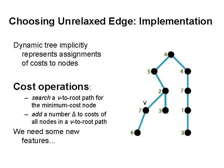
Choosing Unrelaxed Edge: Implementation Dynamic tree implicitly represents assignments of costs to nodes Cost operations: – search a v-to-root path for the minimum-cost node – add a number Δ to costs of all nodes in a v-to-root path We need some new features…

Choosing Unrelaxed Edge Using Dynamic Tree For each non-tree primal edge uv, define σ(uv) = d. T(u) + len(uv) – d. T(v) Measure of how relaxed the edge is. Unrelaxed edges have negative σ values

Choosing Unrelaxed Edge Using Dynamic Tree For each non-tree primal edge uv, define σ(uv) = d. T(u) + len(uv) – d. T(v) Measure of how relaxed the edge is. Unrelaxed edges have negative σ values Dual edges: same σ values as primal edges

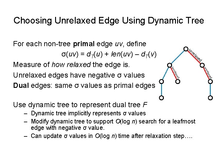
Choosing Unrelaxed Edge Using Dynamic Tree For each non-tree primal edge uv, define σ(uv) = d. T(u) + len(uv) – d. T(v) Measure of how relaxed the edge is. Unrelaxed edges have negative σ values Dual edges: same σ values as primal edges Use dynamic tree to represent dual tree F – Dynamic tree implicitly represents σ values – Modify dynamic tree to support O(log n) search for a leafmost edge with negative σ value. – Can update σ values in O(log n) time after relaxation step….

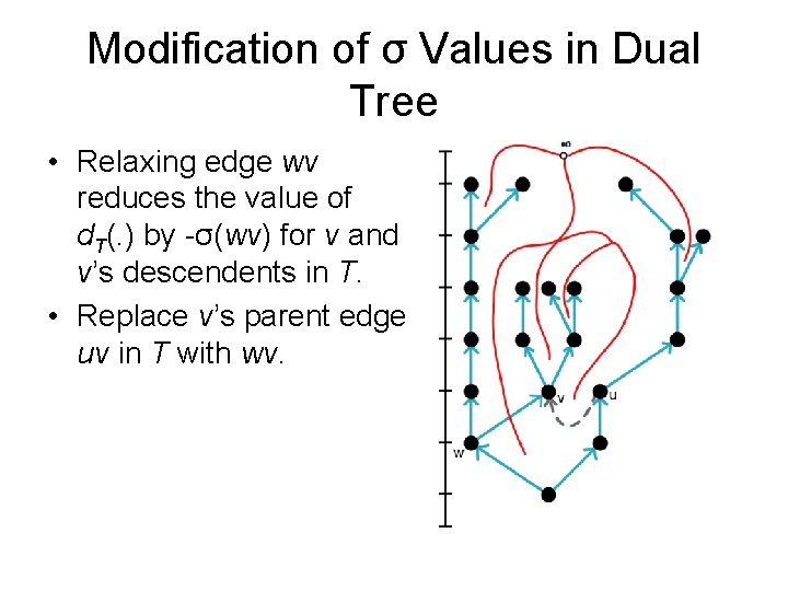
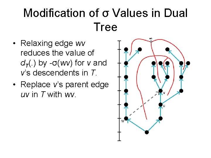
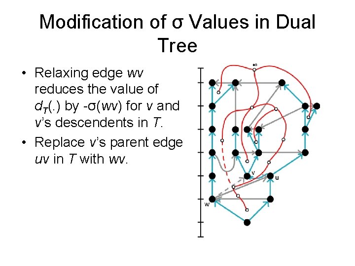
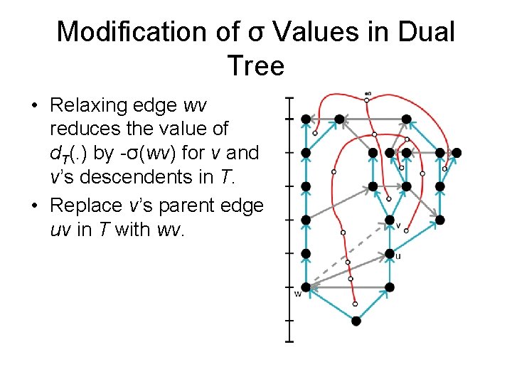
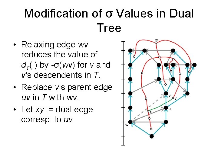
Modification of σ Values in Dual Tree • Relaxing edge wv reduces the value of d. T(. ) by -σ(wv) for v and v’s descendents in T. • Replace v’s parent edge uv in T with wv.

Modification of σ Values in Dual Tree • Relaxing edge wv reduces the value of d. T(. ) by -σ(wv) for v and v’s descendents in T. • Replace v’s parent edge uv in T with wv.

Modification of σ Values in Dual Tree • Relaxing edge wv reduces the value of d. T(. ) by -σ(wv) for v and v’s descendents in T. • Replace v’s parent edge uv in T with wv.

Modification of σ Values in Dual Tree • Relaxing edge wv reduces the value of d. T(. ) by -σ(wv) for v and v’s descendents in T. • Replace v’s parent edge uv in T with wv.

Modification of σ Values in Dual Tree • Relaxing edge wv reduces the value of d. T(. ) by -σ(wv) for v and v’s descendents in T. • Replace v’s parent edge uv in T with wv.

Modification of σ Values in Dual Tree • Relaxing edge wv reduces the value of d. T(. ) by -σ(wv) for v and v’s descendents in T. • Replace v’s parent edge uv in T with wv.

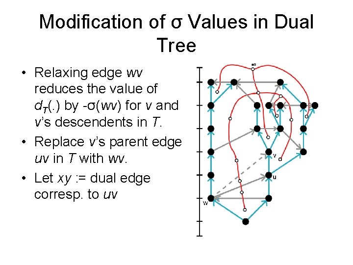
Modification of σ Values in Dual Tree • Relaxing edge wv reduces the value of d. T(. ) by -σ(wv) for v and v’s descendents in T. • Replace v’s parent edge uv in T with wv. • Let xy : = dual edge corresp. to uv

Modification of σ Values in Dual Tree • Relaxing edge wv reduces the value of d. T(. ) by -σ(wv) for v and v’s descendents in T. • Replace v’s parent edge uv in T with wv. • Let xy : = dual edge corresp. to uv

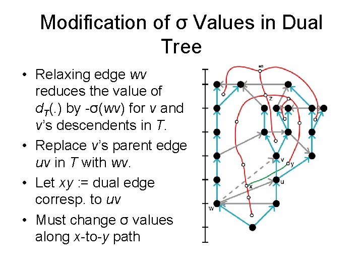
Modification of σ Values in Dual Tree • Relaxing edge wv reduces the value of d. T(. ) by -σ(wv) for v and v’s descendents in T. • Replace v’s parent edge uv in T with wv. • Let xy : = dual edge corresp. to uv • Must change σ values along x-to-y path

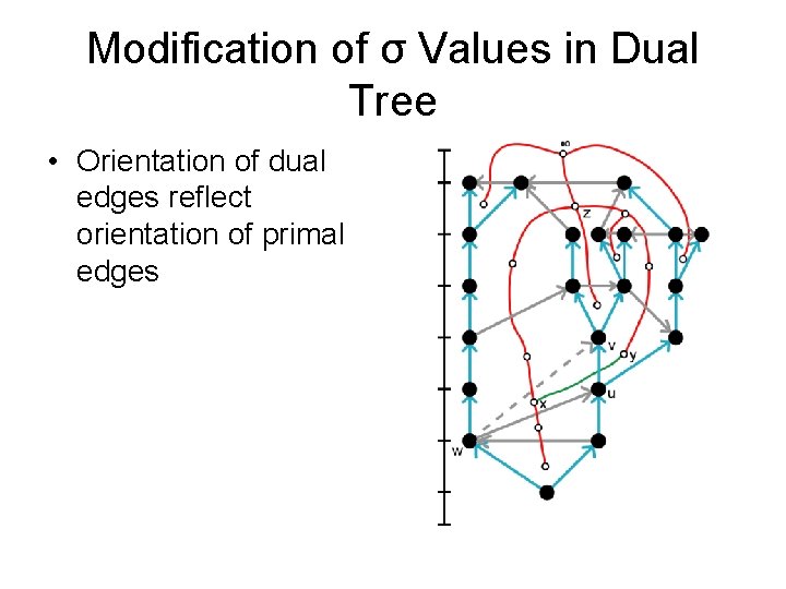
Modification of σ Values in Dual Tree • Orientation of dual edges reflect orientation of primal edges

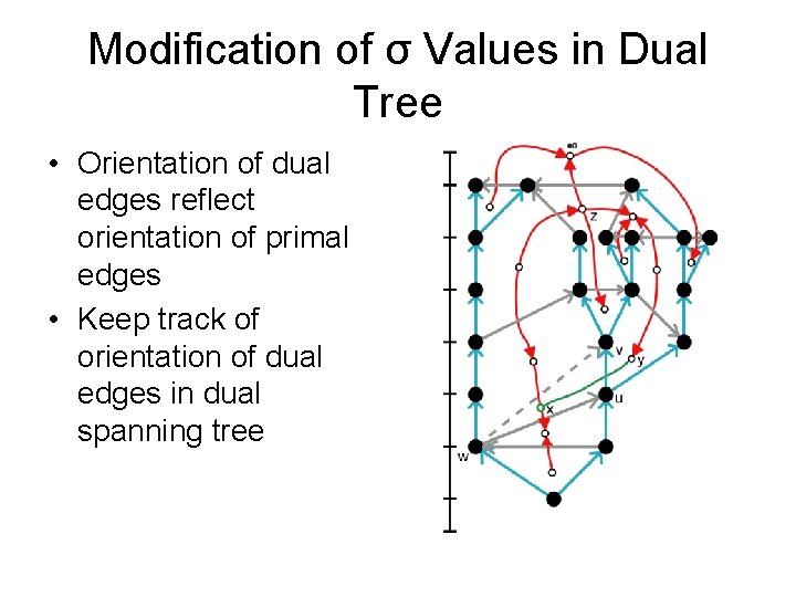
Modification of σ Values in Dual Tree • Orientation of dual edges reflect orientation of primal edges • Keep track of orientation of dual edges in dual spanning tree

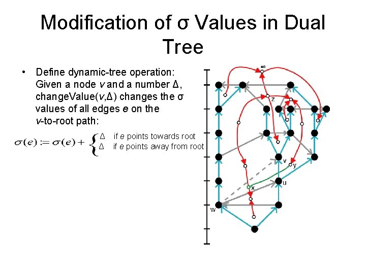
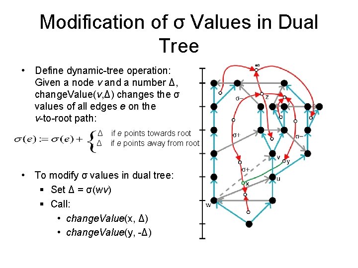
Modification of σ Values in Dual Tree • Define dynamic-tree operation: Given a node v and a number Δ, change. Value(v, Δ) changes the σ values of all edges e on the v-to-root path: Δ -Δ if e points towards root if e points away from root

Modification of σ Values in Dual Tree • Define dynamic-tree operation: Given a node v and a number Δ, change. Value(v, Δ) changes the σ values of all edges e on the v-to-root path: Δ -Δ if e points towards root if e points away from root • To modify σ values in dual tree: § Set Δ = σ(wv) § Call: • change. Value(x, Δ) • change. Value(y, -Δ)

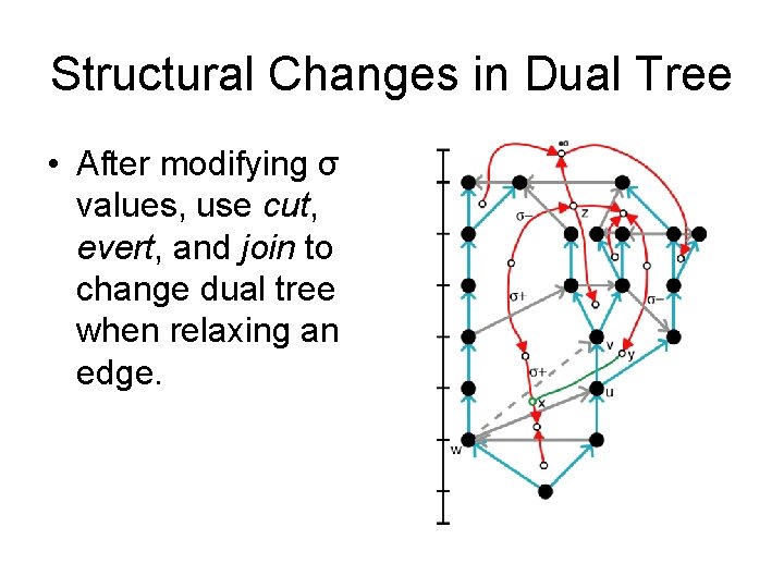
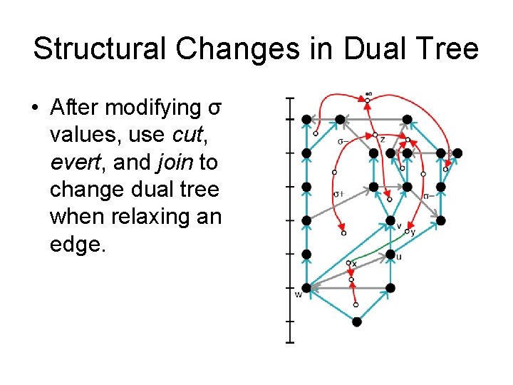
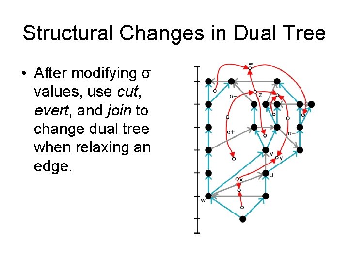
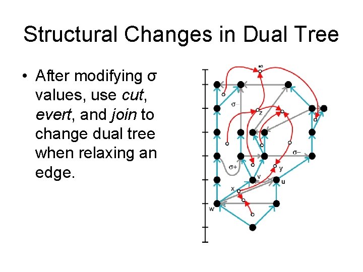
Structural Changes in Dual Tree • After modifying σ values, use cut, evert, and join to change dual tree when relaxing an edge.

Structural Changes in Dual Tree • After modifying σ values, use cut, evert, and join to change dual tree when relaxing an edge.

Structural Changes in Dual Tree • After modifying σ values, use cut, evert, and join to change dual tree when relaxing an edge.

Structural Changes in Dual Tree • After modifying σ values, use cut, evert, and join to change dual tree when relaxing an edge.

Single-Source Algorithm Start with some tree rooted at r. Repeat select a leafmost unrelaxed edge relax it until none exist Questions: • Which tree to start with? (Later. ) • How to find a leafmost edge? Use the dual dynamic tree. • How to bound time required? Each relaxation requires amortized O(log n) time. Need to bound number of relaxations.

Single-Source Algorithm Start with some tree rooted at r. Repeat select a leafmost unrelaxed edge relax it until none exist Questions: • Which tree to start with? (Later. ) • How to find a leafmost edge? Use the dual dynamic tree. • How to bound time required? Each relaxation requires amortized O(log n) time. Need to bound number of relaxations. Theorem: Each edge is relaxed at most once. (Proof later)

Notation: T[v] • For a tree T and a node v, T[v] denotes the root-to-v path in T.

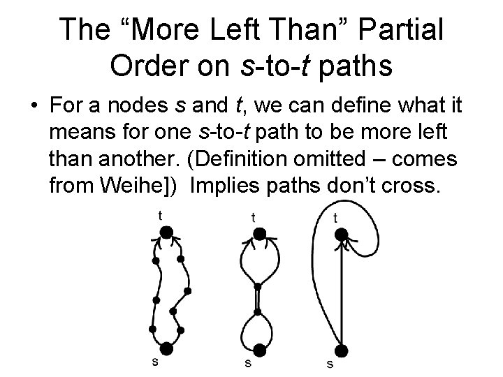
The “More Left Than” Partial Order on s-to-t paths • For a nodes s and t, we can define what it means for one s-to-t path to be more left than another. (Definition omitted – comes from Weihe]) Implies paths don’t cross.

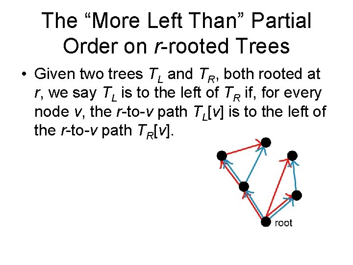
The “More Left Than” Partial Order on r-rooted Trees • Given two trees TL and TR, both rooted at r, we say TL is to the left of TR if, for every node v, the r-to-v path TL[v] is to the left of the r-to-v path TR[v].

Right-First Search [Ripphausen-Lipa, Wagner, Weihe] • Depth-first search where you explore outgoing edges from right to left.

Right-First Search [Ripphausen-Lipa, Wagner, Weihe] • Depth-first search where you explore outgoing edges from right to left.

Right-First Search [Ripphausen-Lipa, Wagner, Weihe] • Depth-first search where you explore outgoing edges from right to left. • The right-first search tree T has the following property: For any node v, the path T[v] is the rightmost root-to-v path.

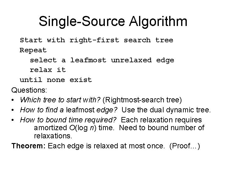
Single-Source Algorithm Start with right-first search tree Repeat select a leafmost unrelaxed edge relax it until none exist Questions: • Which tree to start with? (Rightmost-search tree) • How to find a leafmost edge? Use the dual dynamic tree. • How to bound time required? Each relaxation requires amortized O(log n) time. Need to bound number of relaxations. Theorem: Each edge is relaxed at most once. (Proof…)

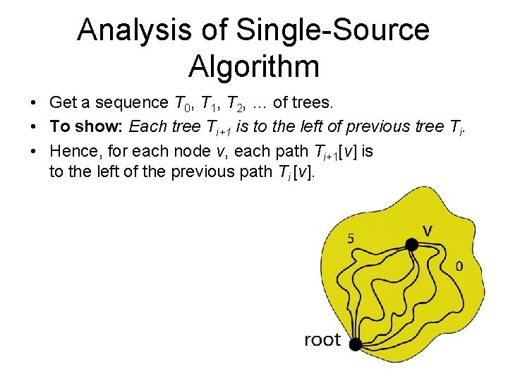
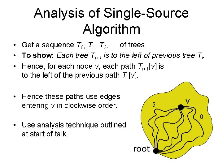
Analysis of Single-Source Algorithm • Get a sequence T 0, T 1, T 2, … of trees. • To show: Each tree Ti+1 is to the left of previous tree Ti. • Hence, for each node v, each path Ti+1[v] is to the left of the previous path Ti [v].

Analysis of Single-Source Algorithm • Get a sequence T 0, T 1, T 2, … of trees. • To show: Each tree Ti+1 is to the left of previous tree Ti. • Hence, for each node v, each path Ti+1[v] is to the left of the previous path Ti [v]. • Hence these paths use edges entering v in clockwise order. • Use analysis technique outlined at start of talk.

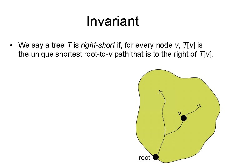
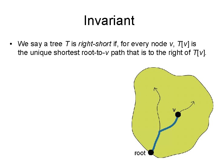
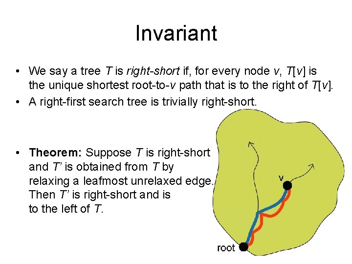
Invariant • We say a tree T is right-short if, for every node v, T[v] is the unique shortest root-to-v path that is to the right of T[v].

Invariant • We say a tree T is right-short if, for every node v, T[v] is the unique shortest root-to-v path that is to the right of T[v].

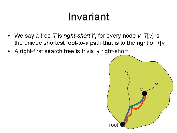
Invariant • We say a tree T is right-short if, for every node v, T[v] is the unique shortest root-to-v path that is to the right of T[v]. • A right-first search tree is trivially right-short.

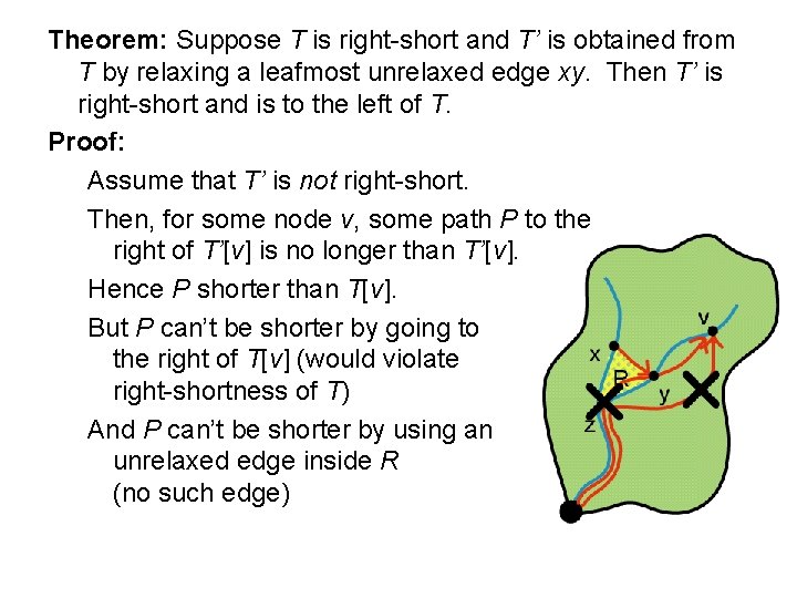
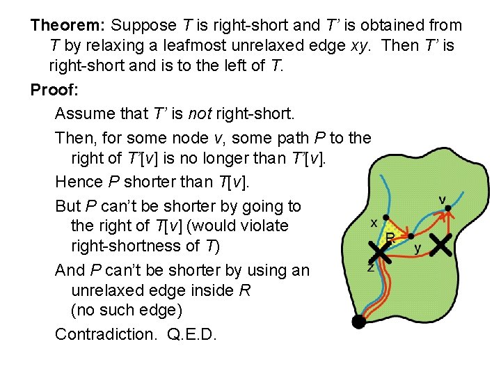
Invariant • We say a tree T is right-short if, for every node v, T[v] is the unique shortest root-to-v path that is to the right of T[v]. • A right-first search tree is trivially right-short. • Theorem: Suppose T is right-short and T’ is obtained from T by relaxing a leafmost unrelaxed edge. Then T’ is right-short and is to the left of T.

Consider an unrelaxed edge xy. Suppose the path T[x] ◦ xy is to the right of T[y]. xy is unrelaxed => T[x] ◦ xy is shorter than T[y] is not the shortest path to the right of T[y]. T is not right-short.

Consider an unrelaxed edge xy. Suppose the path T[x] ◦ xy is to the right of T[y]. xy is unrelaxed => T[x] ◦ xy is shorter than T[y] is not the shortest path to the right of T[y]. T is not right-short. Lemma 1: If T is right-short and xy is unrelaxed then T[x] ◦ xy is to the left of T[y].

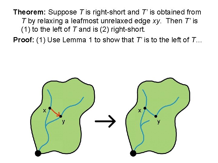
Theorem: Suppose T is right-short and T’ is obtained from T by relaxing a leafmost unrelaxed edge xy. Then T’ is (1) to the left of T and is (2) right-short. Proof: (1) Use Lemma 1 to show that T’ is to the left of T…

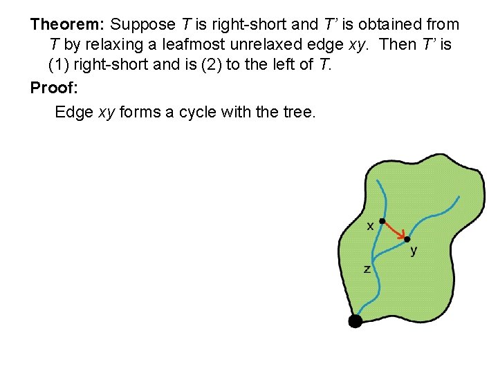
Theorem: Suppose T is right-short and T’ is obtained from T by relaxing a leafmost unrelaxed edge xy. Then T’ is (1) right-short and is (2) to the left of T. Proof: Edge xy forms a cycle with the tree.

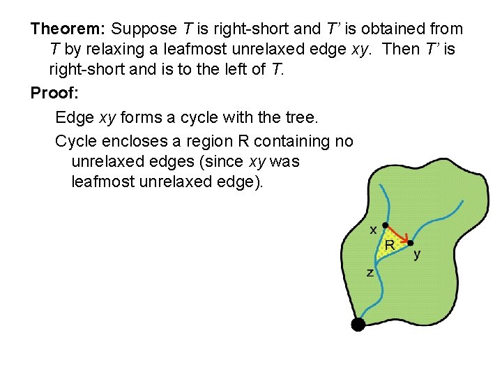
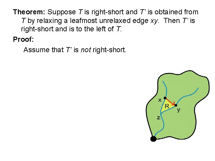
Theorem: Suppose T is right-short and T’ is obtained from T by relaxing a leafmost unrelaxed edge xy. Then T’ is right-short and is to the left of T. Proof: Edge xy forms a cycle with the tree. Cycle encloses a region R containing no unrelaxed edges (since xy was leafmost unrelaxed edge).

Theorem: Suppose T is right-short and T’ is obtained from T by relaxing a leafmost unrelaxed edge xy. Then T’ is right-short and is to the left of T. Proof: Assume that T’ is not right-short.

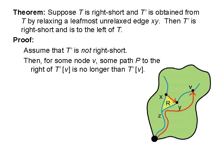
Theorem: Suppose T is right-short and T’ is obtained from T by relaxing a leafmost unrelaxed edge xy. Then T’ is right-short and is to the left of T. Proof: Assume that T’ is not right-short. Then, for some node v, some path P to the right of T’ [v] is no longer than T’ [v].

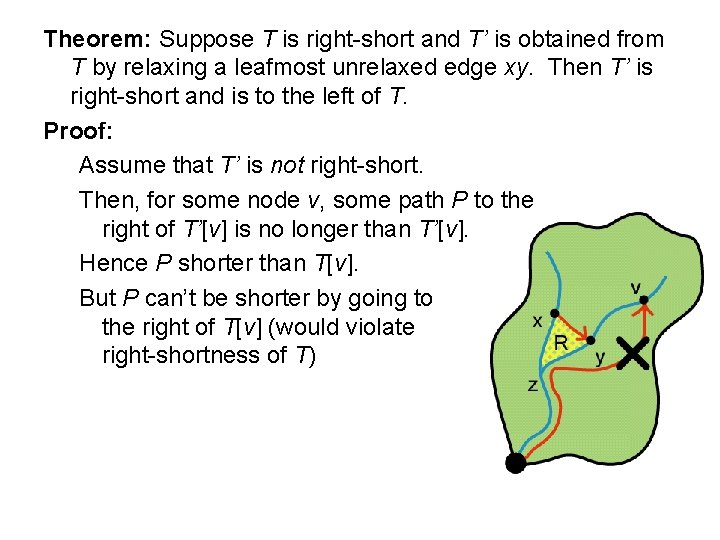
Theorem: Suppose T is right-short and T’ is obtained from T by relaxing a leafmost unrelaxed edge xy. Then T’ is right-short and is to the left of T. Proof: Assume that T’ is not right-short. Then, for some node v, some path P to the right of T’[v] is no longer than T’[v]. Hence P shorter than T[v]. But P can’t be shorter by going to the right of T[v] (would violate right-shortness of T)

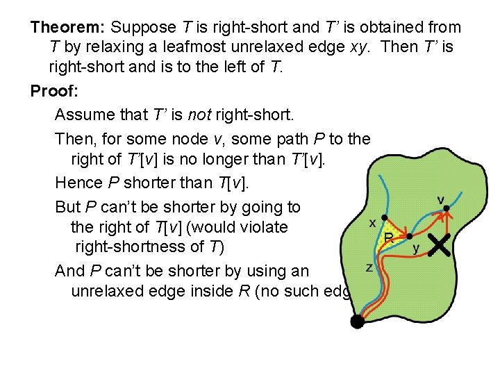
Theorem: Suppose T is right-short and T’ is obtained from T by relaxing a leafmost unrelaxed edge xy. Then T’ is right-short and is to the left of T. Proof: Assume that T’ is not right-short. Then, for some node v, some path P to the right of T’[v] is no longer than T’[v]. Hence P shorter than T[v]. But P can’t be shorter by going to the right of T[v] (would violate right-shortness of T) And P can’t be shorter by using an unrelaxed edge inside R (no such edge)

Theorem: Suppose T is right-short and T’ is obtained from T by relaxing a leafmost unrelaxed edge xy. Then T’ is right-short and is to the left of T. Proof: Assume that T’ is not right-short. Then, for some node v, some path P to the right of T’[v] is no longer than T’[v]. Hence P shorter than T[v]. But P can’t be shorter by going to the right of T[v] (would violate right-shortness of T) And P can’t be shorter by using an unrelaxed edge inside R (no such edge)

Theorem: Suppose T is right-short and T’ is obtained from T by relaxing a leafmost unrelaxed edge xy. Then T’ is right-short and is to the left of T. Proof: Assume that T’ is not right-short. Then, for some node v, some path P to the right of T’[v] is no longer than T’[v]. Hence P shorter than T[v]. But P can’t be shorter by going to the right of T[v] (would violate right-shortness of T) And P can’t be shorter by using an unrelaxed edge inside R (no such edge) Contradiction. Q. E. D.

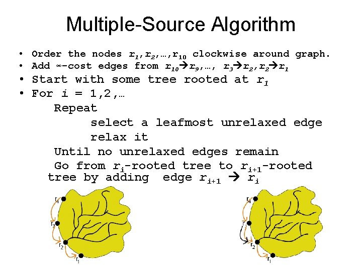
Multiple-Source Algorithm • Order the nodes r 1, r 2, …, r 10 clockwise around graph. • Add ∞-cost edges from r 10 r 9, …, r 3 r 2, r 2 r 1 • Start with some tree rooted at r 1 • For i = 1, 2, … Repeat select a leafmost unrelaxed edge relax it Until no unrelaxed edges remain Go from ri-rooted tree to ri+1 -rooted tree by adding edge ri+1 ri

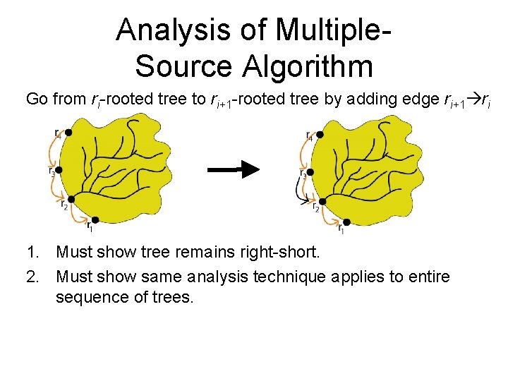
Analysis of Multiple. Source Algorithm Go from ri-rooted tree to ri+1 -rooted tree by adding edge ri+1 ri 1. Must show tree remains right-short. 2. Must show same analysis technique applies to entire sequence of trees.

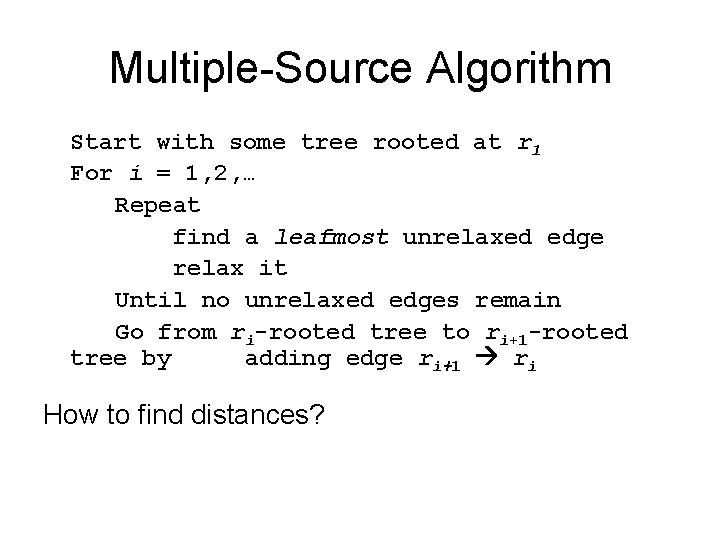
Multiple-Source Algorithm Start with some tree rooted at r 1 For i = 1, 2, … Repeat find a leafmost unrelaxed edge relax it Until no unrelaxed edges remain Go from ri-rooted tree to ri+1 -rooted tree by adding edge ri+1 ri How to find distances?

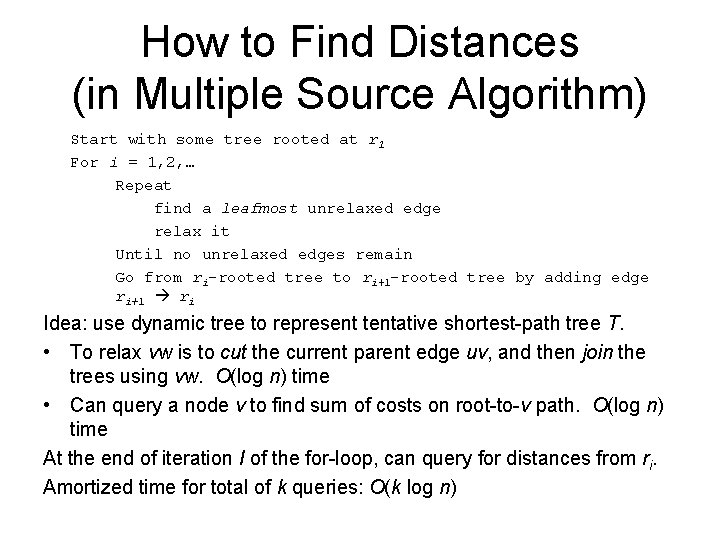
How to Find Distances (in Multiple Source Algorithm) Start with some tree rooted at r 1 For i = 1, 2, … Repeat find a leafmost unrelaxed edge relax it Until no unrelaxed edges remain Go from ri-rooted tree to ri+1 -rooted tree by adding edge ri+1 ri Idea: use dynamic tree to represent tentative shortest-path tree T. • To relax vw is to cut the current parent edge uv, and then join the trees using vw. O(log n) time • Can query a node v to find sum of costs on root-to-v path. O(log n) time At the end of iteration I of the for-loop, can query for distances from ri. Amortized time for total of k queries: O(k log n)

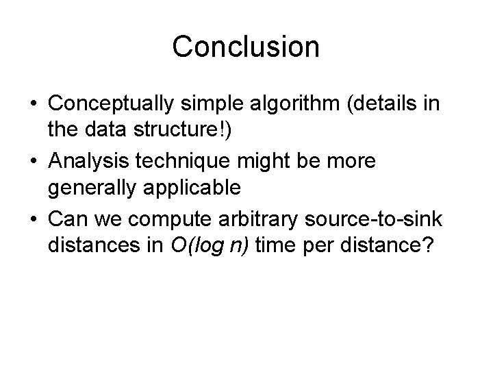
Conclusion • Conceptually simple algorithm (details in the data structure!) • Analysis technique might be more generally applicable • Can we compute arbitrary source-to-sink distances in O(log n) time per distance?