Multiple View Geometry and Stereo Overview Single camera

Multiple View Geometry and Stereo

Overview • Single camera geometry – Recap of Homogenous coordinates – Perspective projection model – Camera calibration • Stereo Reconstruction – Epipolar geometry – Stereo correspondence – Triangulation

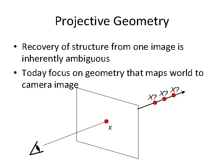
Projective Geometry • Recovery of structure from one image is inherently ambiguous • Today focus on geometry that maps world to camera image X? X? X? x

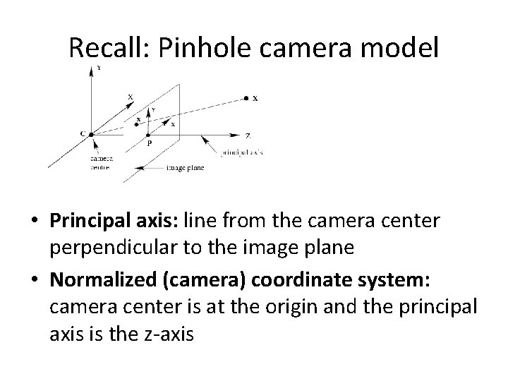
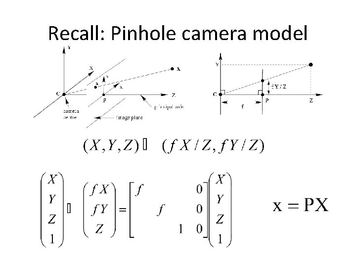
Recall: Pinhole camera model • Principal axis: line from the camera center perpendicular to the image plane • Normalized (camera) coordinate system: camera center is at the origin and the principal axis is the z-axis

Recall: Pinhole camera model

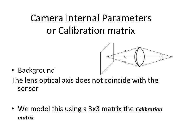
Camera Internal Parameters or Calibration matrix • Background The lens optical axis does not coincide with the sensor • We model this using a 3 x 3 matrix the Calibration matrix

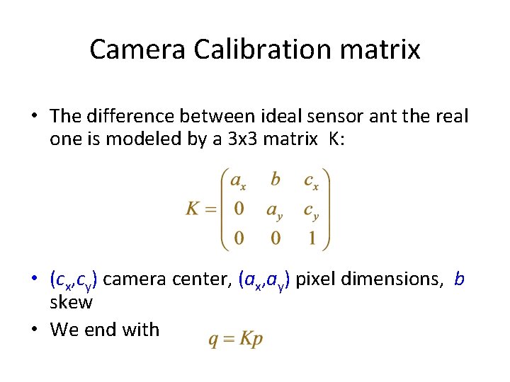
Camera Calibration matrix • The difference between ideal sensor ant the real one is modeled by a 3 x 3 matrix K: • (cx, cy) camera center, (ax, ay) pixel dimensions, b skew • We end with

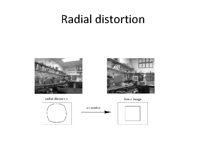
Radial distortion

Camera parameters • Intrinsic parameters – Principal point coordinates – Focal length – Pixel magnification factors – Skew (non-rectangular pixels) – Radial distortion • Extrinsic parameters – Rotation and translation relative to world coordinate system

Scenarios The two images can arise from • A stereo rig consisting of two cameras or – the two images are acquired simultaneously • A single moving camera (static scene) – the two images are acquired sequentially The two scenarios are geometrically equivalent

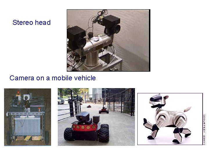
Stereo head Camera on a mobile vehicle

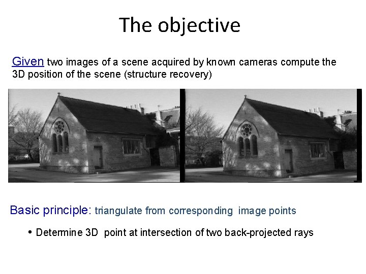
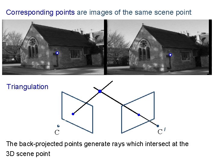
The objective Given two images of a scene acquired by known cameras compute the 3 D position of the scene (structure recovery) Basic principle: triangulate from corresponding image points • Determine 3 D point at intersection of two back-projected rays

Corresponding points are images of the same scene point Triangulation C C/ The back-projected points generate rays which intersect at the 3 D scene point

An algorithm for stereo reconstruction 1. For each point in the first image determine the corresponding point in the second image (this is a search problem) 2. For each pair of matched points determine the 3 D point by triangulation (this is an estimation problem)

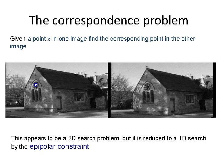
The correspondence problem Given a point x in one image find the corresponding point in the other image This appears to be a 2 D search problem, but it is reduced to a 1 D search by the epipolar constraint

Outline 1. Epipolar geometry • • the geometry of two cameras reduces the correspondence problem to a line search 2. Stereo correspondence algorithms 3. Triangulation

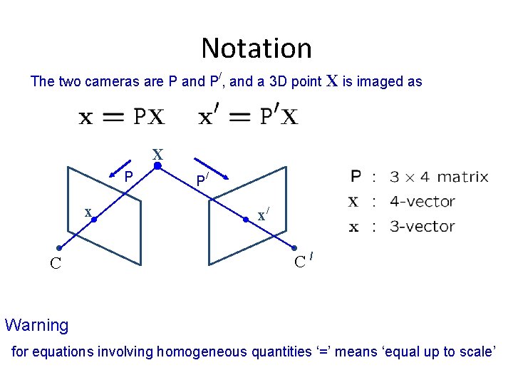
Notation / The two cameras are P and P , and a 3 D point X is imaged as X P x C P/ x/ C/ Warning for equations involving homogeneous quantities ‘=’ means ‘equal up to scale’

Epipolar geometry

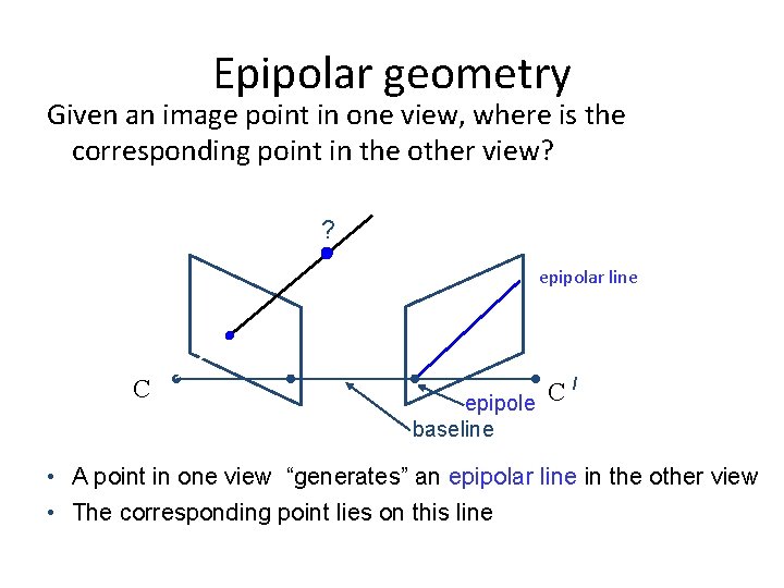
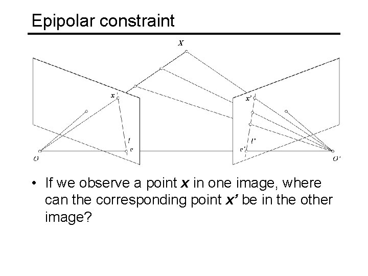
Epipolar geometry Given an image point in one view, where is the corresponding point in the other view? ? epipolar line C / C epipole baseline • A point in one view “generates” an epipolar line in the other view • The corresponding point lies on this line

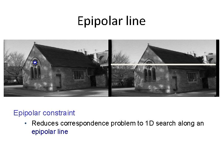
Epipolar line Epipolar constraint • Reduces correspondence problem to 1 D search along an epipolar line

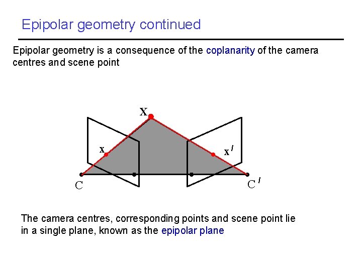
Epipolar geometry continued Epipolar geometry is a consequence of the coplanarity of the camera centres and scene point X x C x/ C/ The camera centres, corresponding points and scene point lie in a single plane, known as the epipolar plane

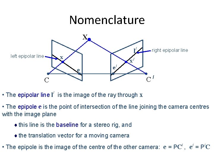
Nomenclature X left epipolar line l/ x right epipolar line x/ e e/ C C/ • The epipolar line l/ is the image of the ray through x • The epipole e is the point of intersection of the line joining the camera centres with the image plane this line is the baseline for a stereo rig, and the translation vector for a moving camera • The epipole is the image of the centre of the other camera: e = PC/ , e/ = P/C

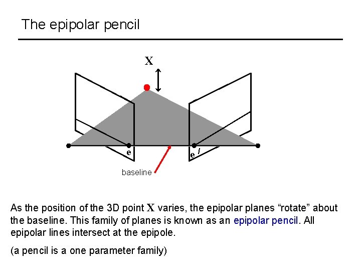
The epipolar pencil X e e / baseline As the position of the 3 D point X varies, the epipolar planes “rotate” about the baseline. This family of planes is known as an epipolar pencil. All epipolar lines intersect at the epipole. (a pencil is a one parameter family)

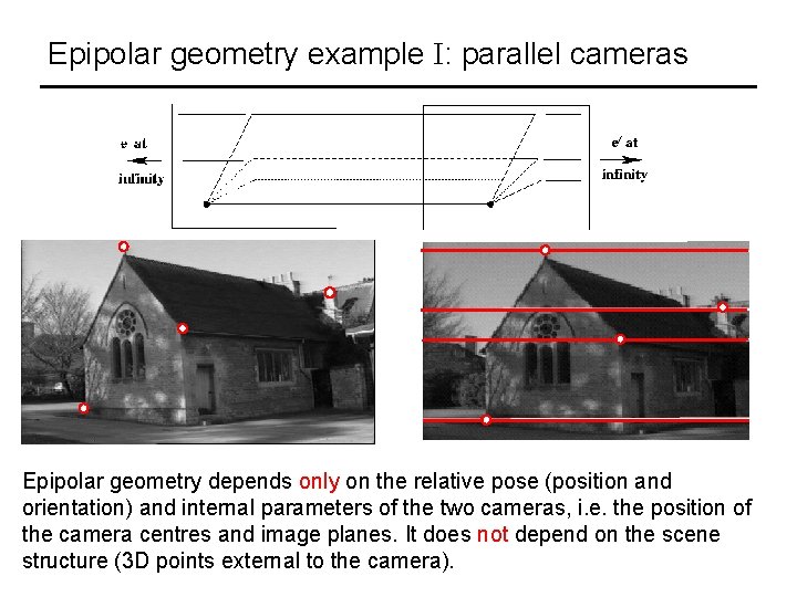
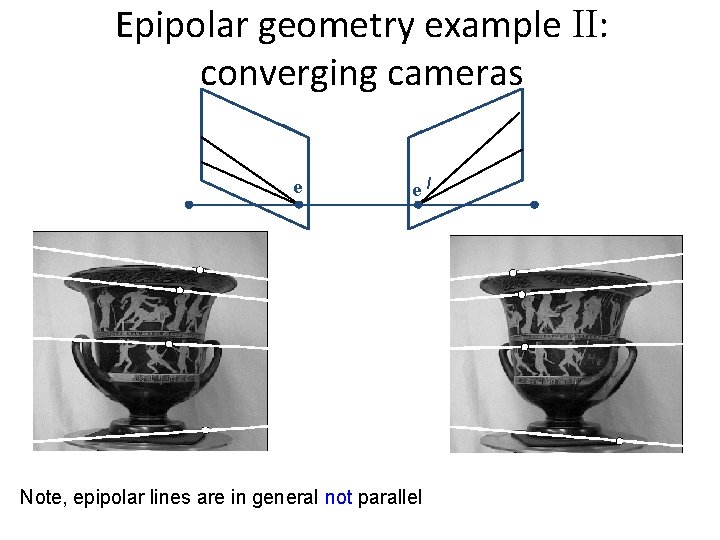
Epipolar geometry example I: parallel cameras Epipolar geometry depends only on the relative pose (position and orientation) and internal parameters of the two cameras, i. e. the position of the camera centres and image planes. It does not depend on the scene structure (3 D points external to the camera).

Epipolar geometry example II: converging cameras e e Note, epipolar lines are in general not parallel /

Epipolar constraint X x x’ • If we observe a point x in one image, where can the corresponding point x’ be in the other image?

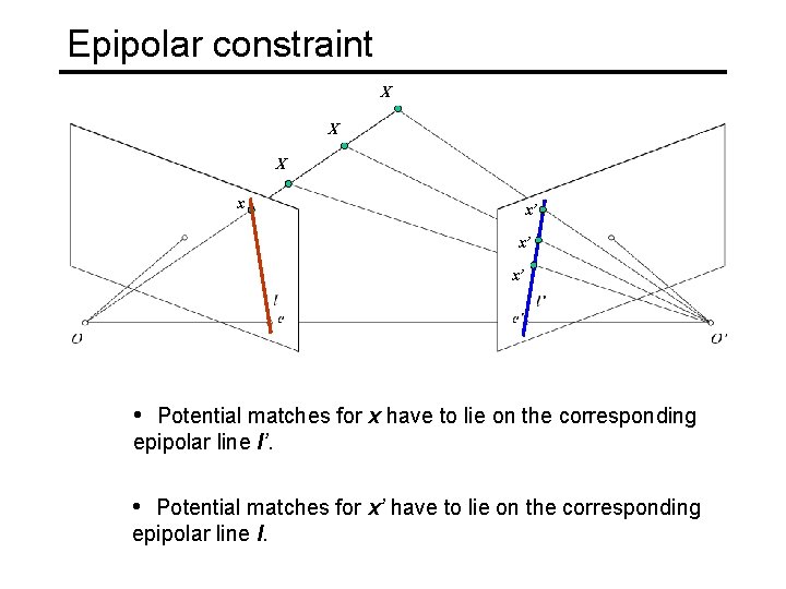
Epipolar constraint X X X x x’ x’ x’ • Potential matches for x have to lie on the corresponding epipolar line l’. • Potential matches for x’ have to lie on the corresponding epipolar line l.

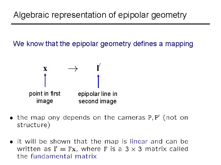
Algebraic representation of epipolar geometry We know that the epipolar geometry defines a mapping / x l point in first image epipolar line in second image

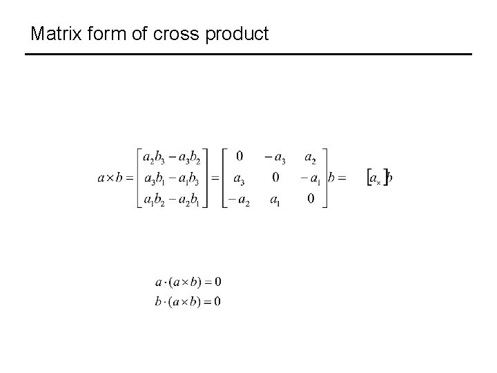
Matrix form of cross product

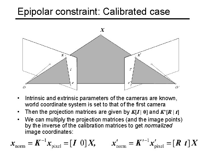
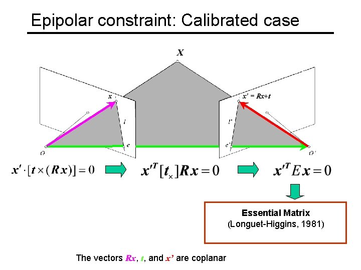
Epipolar constraint: Calibrated case X x x’ • Intrinsic and extrinsic parameters of the cameras are known, world coordinate system is set to that of the first camera • Then the projection matrices are given by K[I | 0] and K’[R | t] • We can multiply the projection matrices (and the image points) by the inverse of the calibration matrices to get normalized image coordinates:

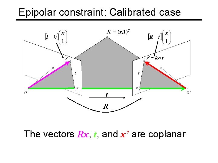
Epipolar constraint: Calibrated case X = (x, 1)T x x’ = Rx+t t R The vectors Rx, t, and x’ are coplanar

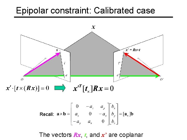
Epipolar constraint: Calibrated case X x x’ = Rx+t Recall: The vectors Rx, t, and x’ are coplanar

Epipolar constraint: Calibrated case X x x’ = Rx+t Essential Matrix (Longuet-Higgins, 1981) The vectors Rx, t, and x’ are coplanar

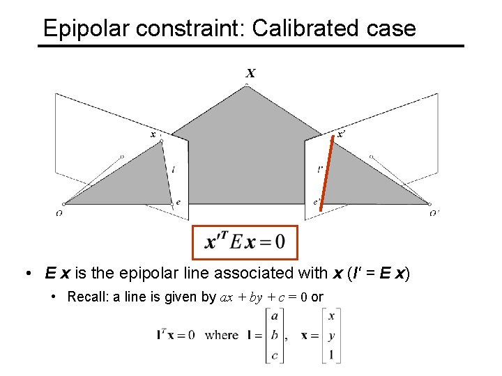
Epipolar constraint: Calibrated case X x x’ • E x is the epipolar line associated with x (l' = E x) • Recall: a line is given by ax + by + c = 0 or

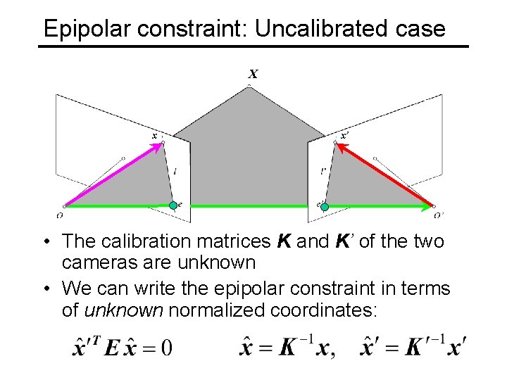
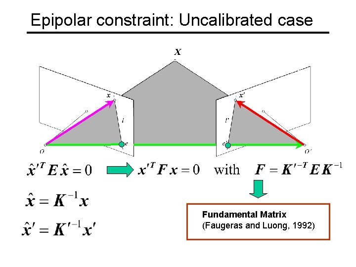
Epipolar constraint: Uncalibrated case X x x’ • The calibration matrices K and K’ of the two cameras are unknown • We can write the epipolar constraint in terms of unknown normalized coordinates:

Epipolar constraint: Uncalibrated case X x x’ Fundamental Matrix (Faugeras and Luong, 1992)

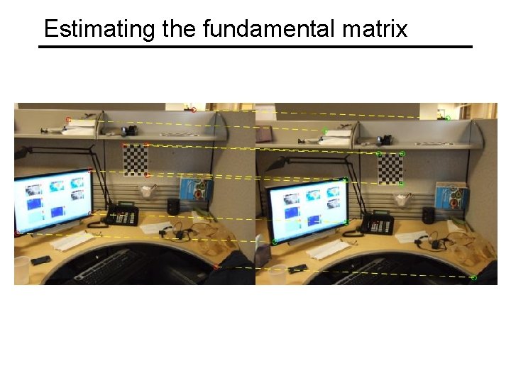
Estimating the fundamental matrix

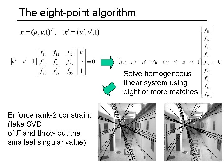
The eight-point algorithm Solve homogeneous linear system using eight or more matches Enforce rank-2 constraint (take SVD of F and throw out the smallest singular value)

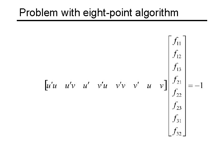
Problem with eight-point algorithm

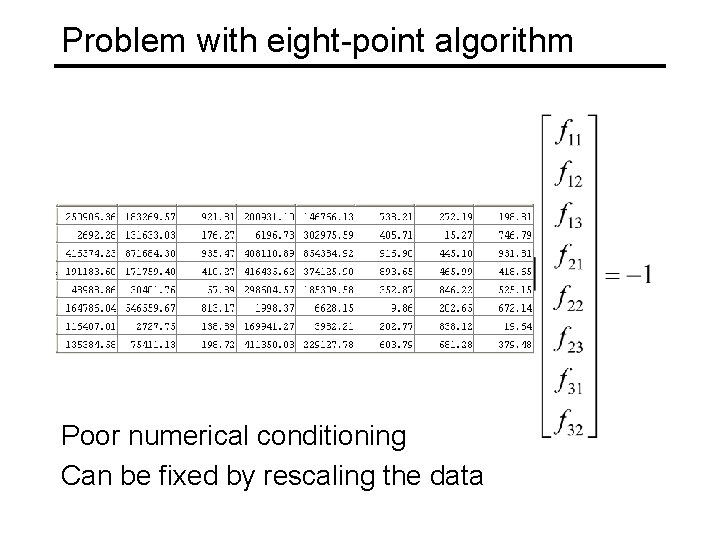
Problem with eight-point algorithm Poor numerical conditioning Can be fixed by rescaling the data

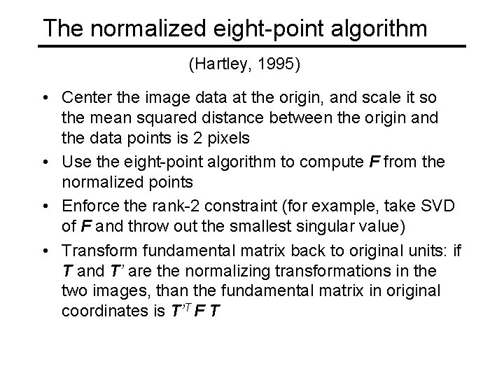
The normalized eight-point algorithm (Hartley, 1995) • Center the image data at the origin, and scale it so the mean squared distance between the origin and the data points is 2 pixels • Use the eight-point algorithm to compute F from the normalized points • Enforce the rank-2 constraint (for example, take SVD of F and throw out the smallest singular value) • Transform fundamental matrix back to original units: if T and T’ are the normalizing transformations in the two images, than the fundamental matrix in original coordinates is T’T F T

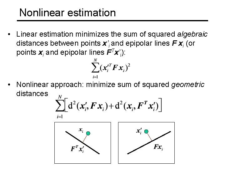
Nonlinear estimation • Linear estimation minimizes the sum of squared algebraic distances between points x’i and epipolar lines F xi (or points xi and epipolar lines FTx’i): • Nonlinear approach: minimize sum of squared geometric distances xi

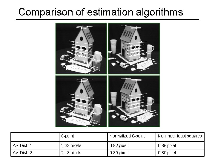
Comparison of estimation algorithms 8 -point Normalized 8 -point Nonlinear least squares Av. Dist. 1 2. 33 pixels 0. 92 pixel 0. 86 pixel Av. Dist. 2 2. 18 pixels 0. 85 pixel 0. 80 pixel

Stereo correspondence algorithms

Stereo correspondence algorithms

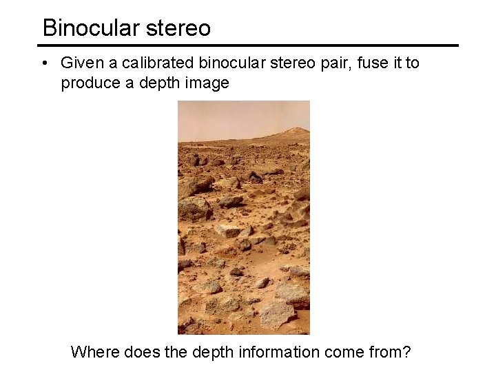
Binocular stereo • Given a calibrated binocular stereo pair, fuse it to produce a depth image Where does the depth information come from?

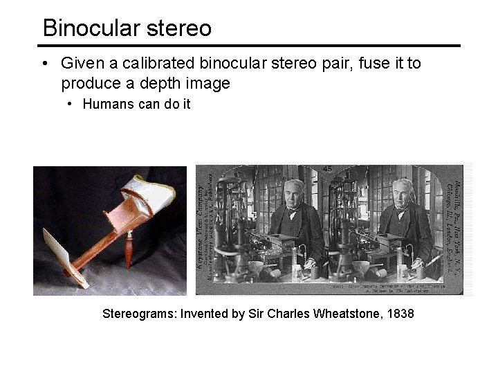
Binocular stereo • Given a calibrated binocular stereo pair, fuse it to produce a depth image • Humans can do it Stereograms: Invented by Sir Charles Wheatstone, 1838

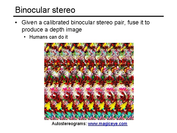
Binocular stereo • Given a calibrated binocular stereo pair, fuse it to produce a depth image • Humans can do it Autostereograms: www. magiceye. com

Stereo Assumes (two) cameras. Known positions. Recover depth.

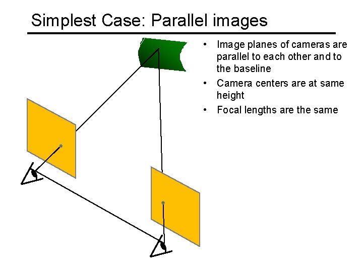
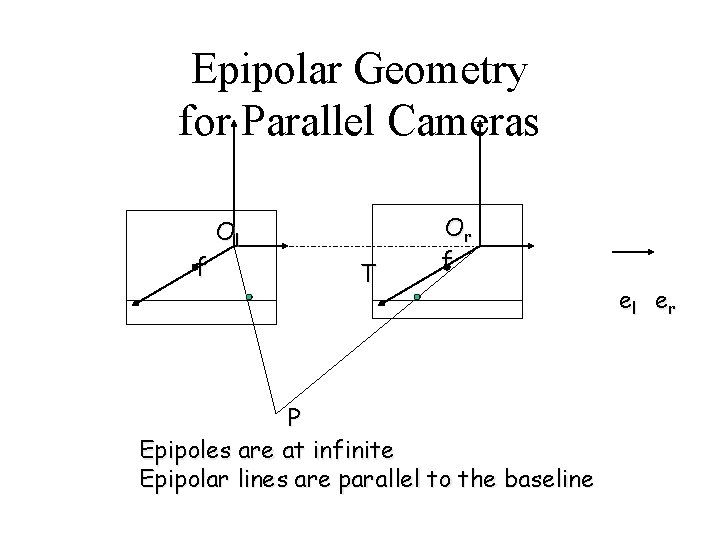
Simplest Case: Parallel images • Image planes of cameras are parallel to each other and to the baseline • Camera centers are at same height • Focal lengths are the same

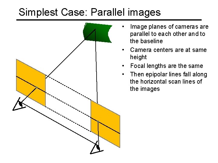
Simplest Case: Parallel images • Image planes of cameras are parallel to each other and to the baseline • Camera centers are at same height • Focal lengths are the same • Then epipolar lines fall along the horizontal scan lines of the images

Simplest Case • • Image planes of cameras are parallel. Focal points are at same height. Focal lengths same. Then, epipolar lines are horizontal scan lines.

Epipolar Geometry for Parallel Cameras f Ol T Or f P Epipoles are at infinite Epipolar lines are parallel to the baseline el er

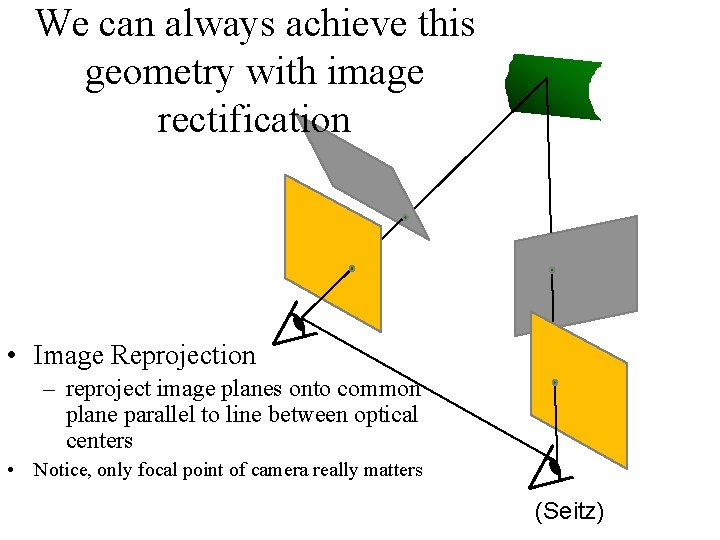
We can always achieve this geometry with image rectification • Image Reprojection – reproject image planes onto common plane parallel to line between optical centers • Notice, only focal point of camera really matters (Seitz)

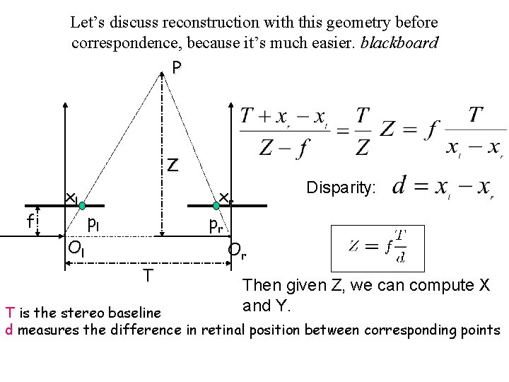
Let’s discuss reconstruction with this geometry before correspondence, because it’s much easier. blackboard P Z f xl Disparity: xr pl pr Ol Or T Then given Z, we can compute X and Y. T is the stereo baseline d measures the difference in retinal position between corresponding points

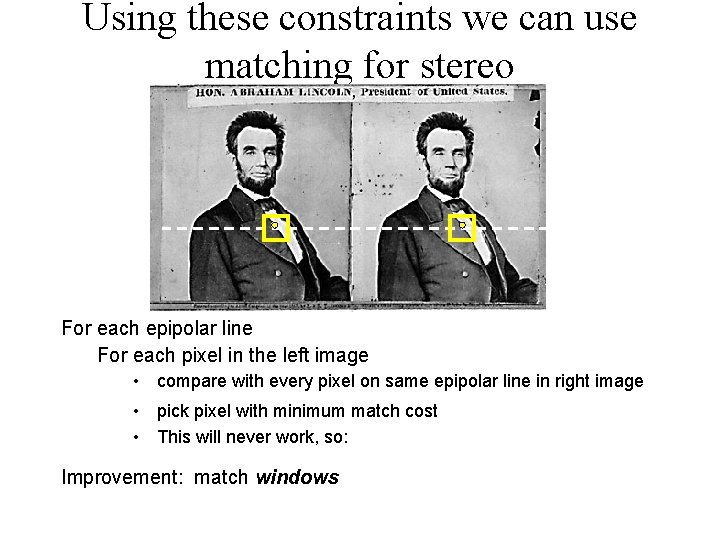
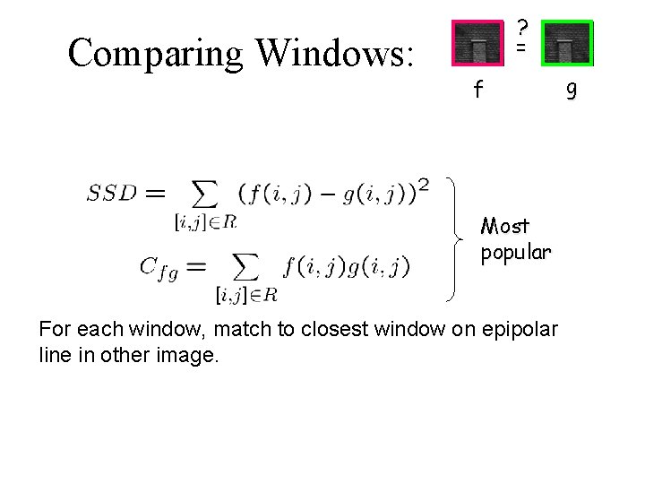
Using these constraints we can use matching for stereo For each epipolar line For each pixel in the left image • compare with every pixel on same epipolar line in right image • pick pixel with minimum match cost • This will never work, so: Improvement: match windows

Comparing Windows: ? = f Most popular For each window, match to closest window on epipolar line in other image. g

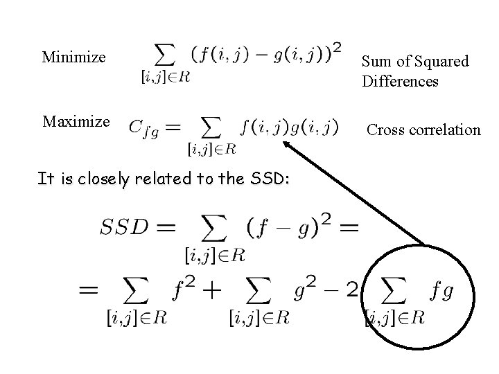
Minimize Maximize It is closely related to the SSD: Sum of Squared Differences Cross correlation

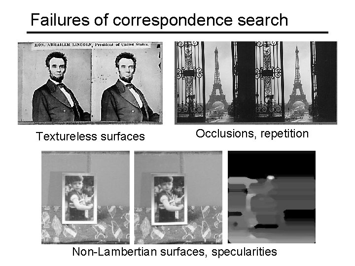
Failures of correspondence search Textureless surfaces Occlusions, repetition Non-Lambertian surfaces, specularities

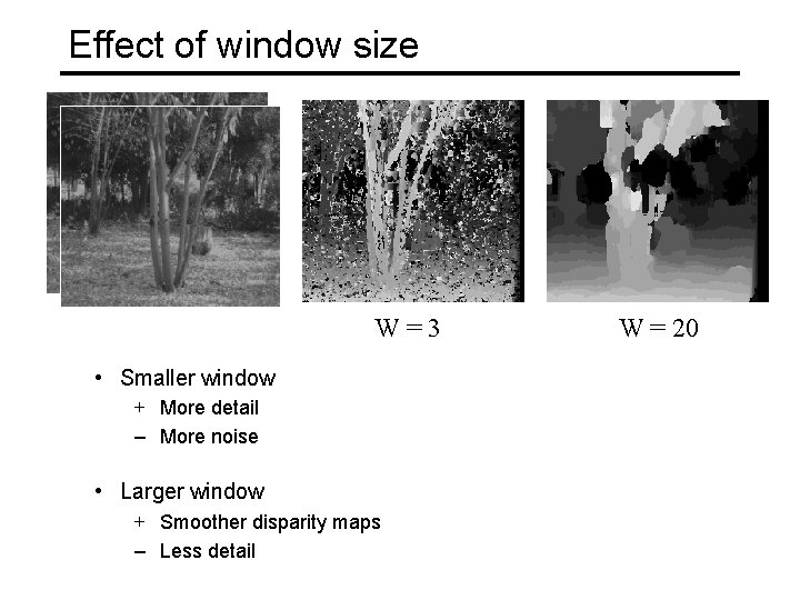
Effect of window size W=3 • Smaller window + More detail – More noise • Larger window + Smoother disparity maps – Less detail W = 20

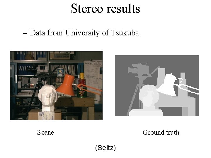
Stereo results – Data from University of Tsukuba Scene Ground truth (Seitz)

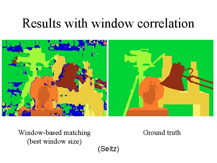
Results with window correlation Window-based matching (best window size) Ground truth (Seitz)

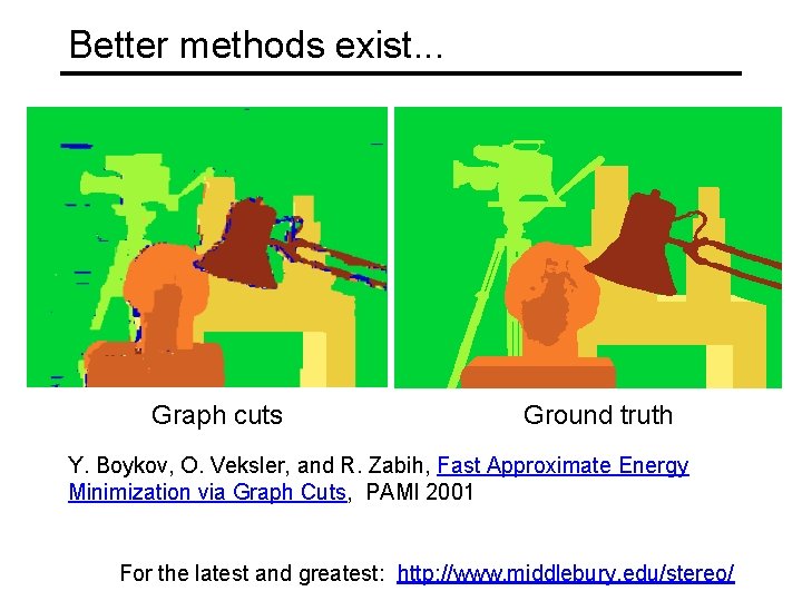
Better methods exist. . . Graph cuts Ground truth Y. Boykov, O. Veksler, and R. Zabih, Fast Approximate Energy Minimization via Graph Cuts, PAMI 2001 For the latest and greatest: http: //www. middlebury. edu/stereo/

How can we improve window-based matching? • The similarity constraint is local (each reference window is matched independently) • Need to enforce non-local correspondence constraints

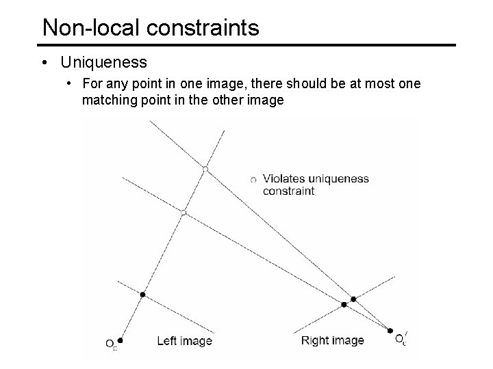
Non-local constraints • Uniqueness • For any point in one image, there should be at most one matching point in the other image

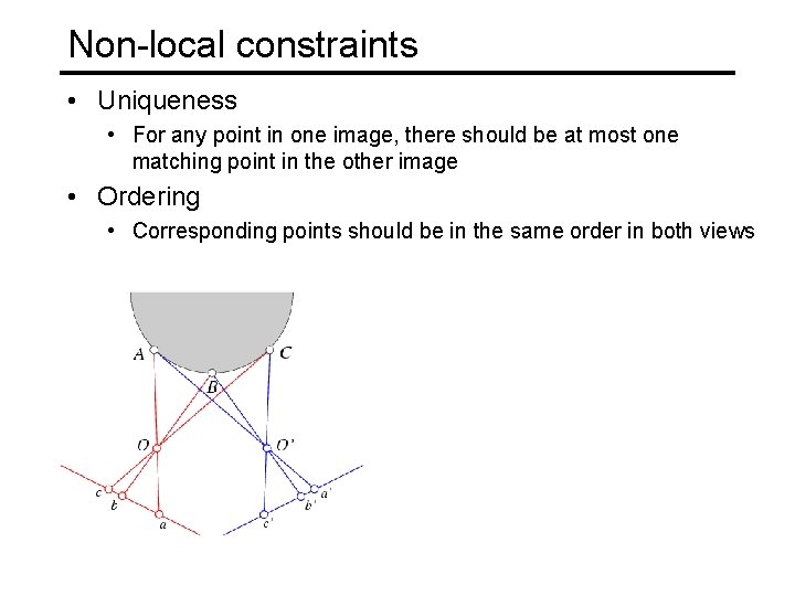
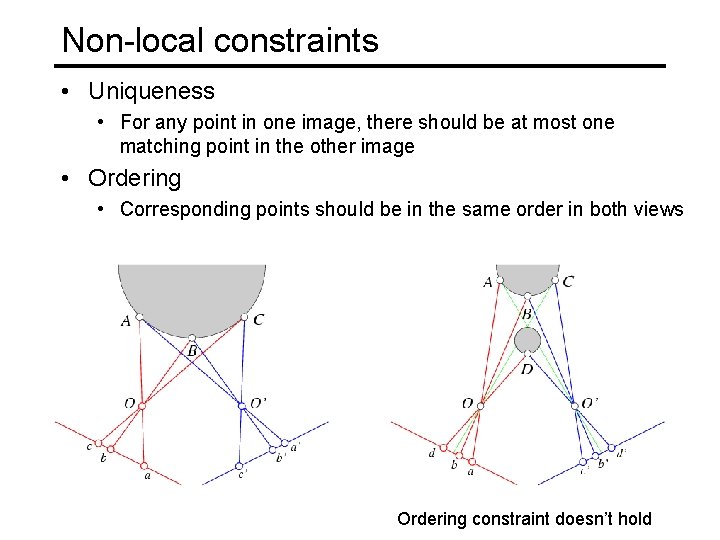
Non-local constraints • Uniqueness • For any point in one image, there should be at most one matching point in the other image • Ordering • Corresponding points should be in the same order in both views

Non-local constraints • Uniqueness • For any point in one image, there should be at most one matching point in the other image • Ordering • Corresponding points should be in the same order in both views Ordering constraint doesn’t hold

Non-local constraints • Uniqueness • For any point in one image, there should be at most one matching point in the other image • Ordering • Corresponding points should be in the same order in both views • Smoothness • We expect disparity values to change slowly (for the most part)

Ordering constraint enables dynamic programming. • If we match pixel i in image 1 to pixel j in image 2, no matches that follow will affect which are the best preceding matches. • Example with pixels (a la Cox et al. ).

Smoothness constraint • Smoothness: disparity usually doesn’t change too quickly. – Unfortunately, this makes the problem 2 D again. – Solved with a host of graph algorithms, Markov Random Fields, Belief Propagation, ….

Scanline stereo • Try to coherently match pixels on the entire scanline • Different scanlines are still optimized independently Left image Right image

“Shortest paths” for scan-line stereo Left image Right occlusion Left occlusion q t s co rre sp on d en ce p Can be implemented with dynamic programming Ohta & Kanade ’ 85, Cox et al. ‘ 96 Slide credit: Y. Boykov

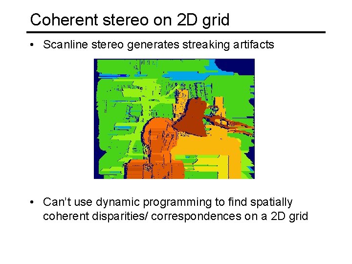
Coherent stereo on 2 D grid • Scanline stereo generates streaking artifacts • Can’t use dynamic programming to find spatially coherent disparities/ correspondences on a 2 D grid

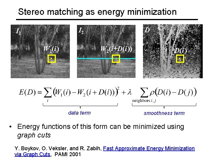
Stereo matching as energy minimization I 2 I 1 W 1(i ) D W 2(i+D(i )) data term D(i ) smoothness term • Energy functions of this form can be minimized using graph cuts Y. Boykov, O. Veksler, and R. Zabih, Fast Approximate Energy Minimization via Graph Cuts, PAMI 2001

Summary • First, we understand constraints that make the problem solvable. – Some are hard, like epipolar constraint. • Ordering isn’t a hard constraint, but most useful when treated like one. – Some are soft, like pixel intensities are similar, disparities usually change slowly. • Then we find optimization method. – Which ones we can use depends on which constraints we pick.