Multiple Sequence Alignment Evolution at the DNA level

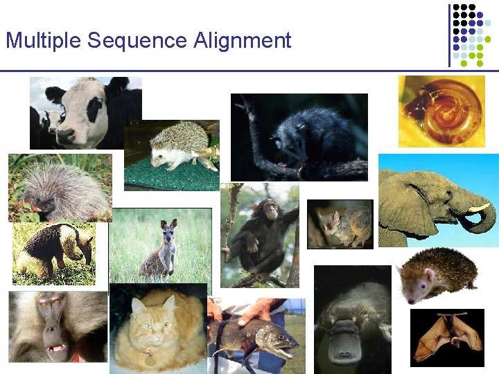
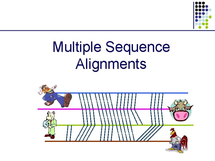
Multiple Sequence Alignment

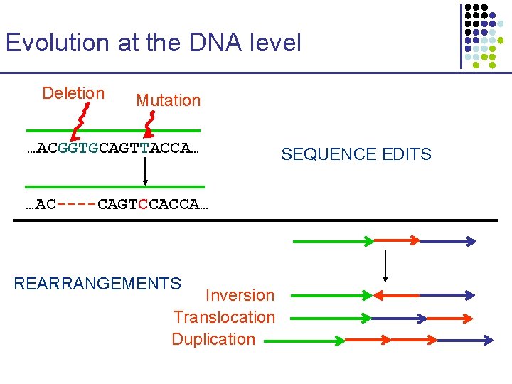
Evolution at the DNA level Deletion Mutation …ACGGTGCAGTTACCA… …AC----CAGTCCACCA… REARRANGEMENTS Inversion Translocation Duplication SEQUENCE EDITS

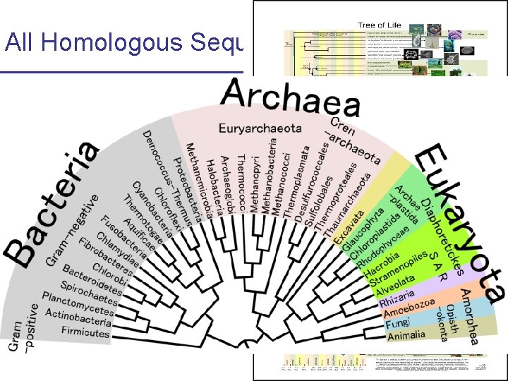
All Homologous Sequences Coalesce Y-chromosome coalescence http: //webvision. umh. es/webvision/Evolution. %20 PART%20 II. html

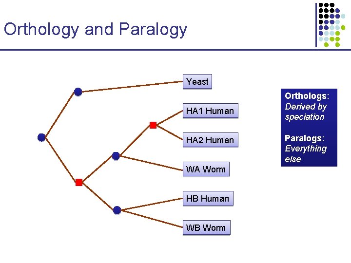
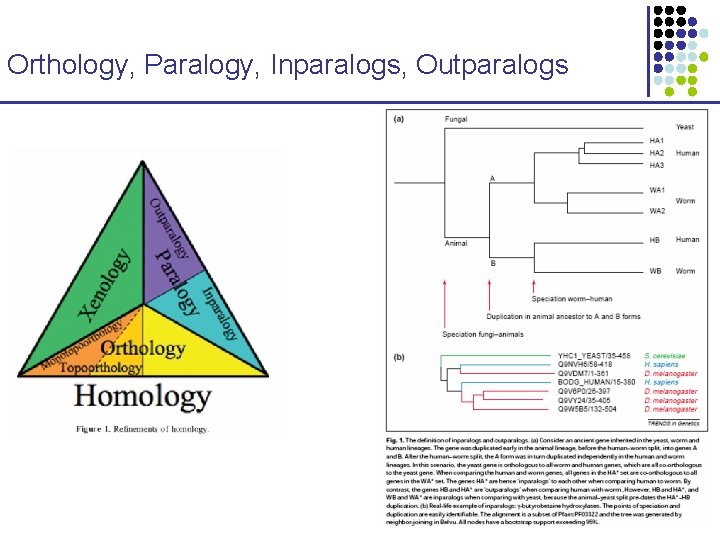
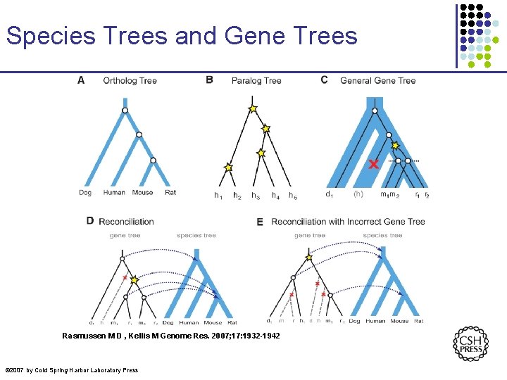
Orthology and Paralogy Yeast HA 1 Human HA 2 Human WA Worm HB Human WB Worm Orthologs: Derived by speciation Paralogs: Everything else

Orthology, Paralogy, Inparalogs, Outparalogs

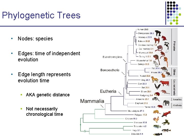
Phylogenetic Trees • Nodes: species • Edges: time of independent evolution • Edge length represents evolution time § AKA genetic distance § Not necessarily chronological time

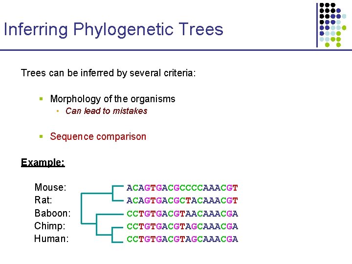
Inferring Phylogenetic Trees can be inferred by several criteria: § Morphology of the organisms • Can lead to mistakes § Sequence comparison Example: Mouse: Rat: Baboon: Chimp: Human: ACAGTGACGCCCCAAACGT ACAGTGACGCTACAAACGT CCTGTGACGTAACAAACGA CCTGTGACGTAGCAAACGA

Distance Between Two Sequences Basic principle: • Distance proportional to degree of independent sequence evolution Given sequences xi, xj, dij = distance between the two sequences One possible definition: dij = fraction f of sites u where xi[u] xj[u] Better scores are derived by modeling evolution as a continuous change process

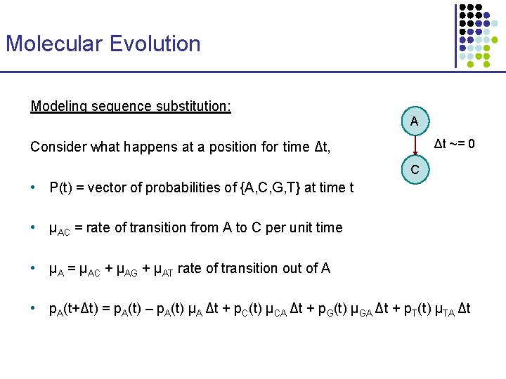
Molecular Evolution Modeling sequence substitution: A Δt ~= 0 Consider what happens at a position for time Δt, C • P(t) = vector of probabilities of {A, C, G, T} at time t • μAC = rate of transition from A to C per unit time • μA = μAC + μAG + μAT rate of transition out of A • p. A(t+Δt) = p. A(t) – p. A(t) μA Δt + p. C(t) μCA Δt + p. G(t) μGA Δt + p. T(t) μTA Δt

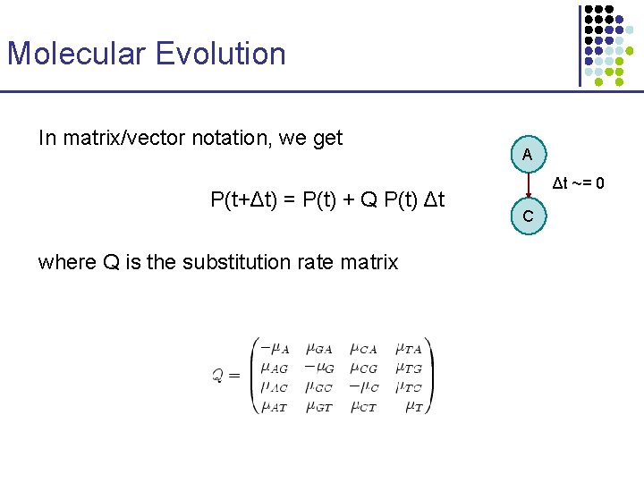
Molecular Evolution In matrix/vector notation, we get P(t+Δt) = P(t) + Q P(t) Δt where Q is the substitution rate matrix A Δt ~= 0 C

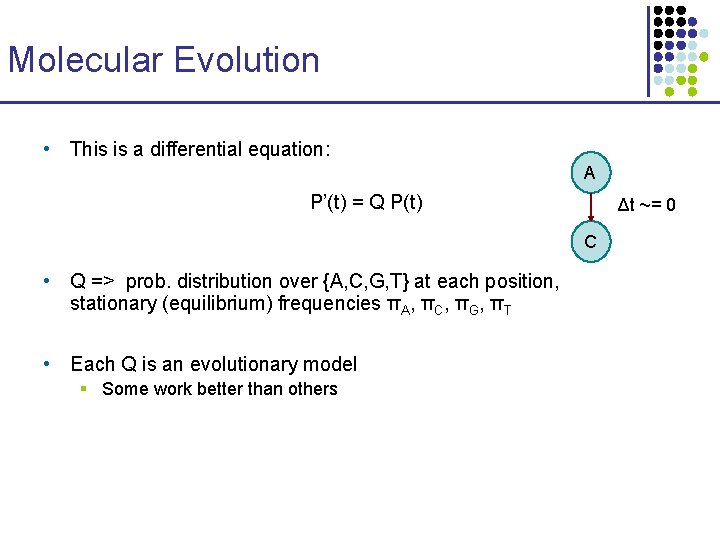
Molecular Evolution • This is a differential equation: A P’(t) = Q P(t) Δt ~= 0 C • Q => prob. distribution over {A, C, G, T} at each position, stationary (equilibrium) frequencies πA, πC, πG, πT • Each Q is an evolutionary model § Some work better than others

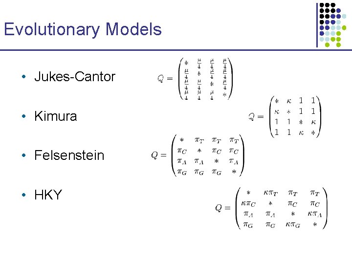
Evolutionary Models • Jukes-Cantor • Kimura • Felsenstein • HKY

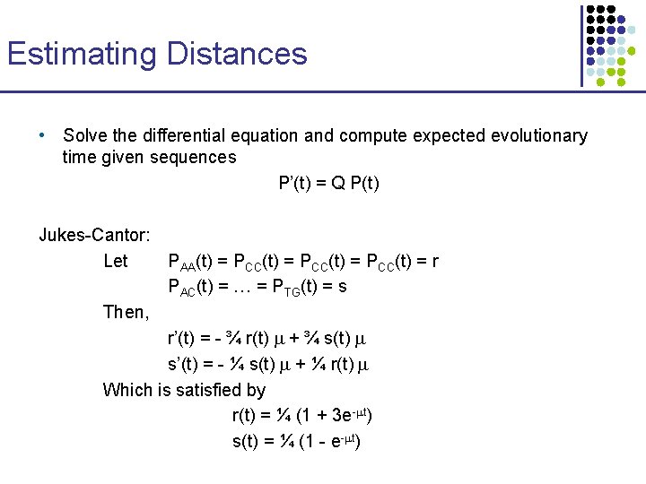
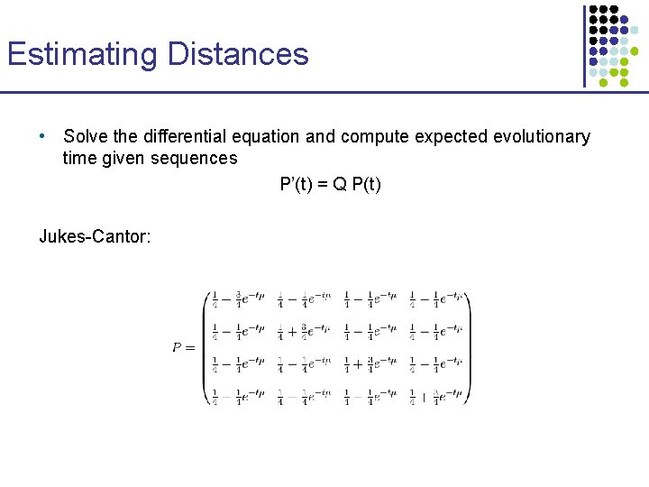
Estimating Distances • Solve the differential equation and compute expected evolutionary time given sequences P’(t) = Q P(t) Jukes-Cantor: Let PAA(t) = PCC(t) = r PAC(t) = … = PTG(t) = s Then, r’(t) = - ¾ r(t) m + ¾ s(t) m s’(t) = - ¼ s(t) m + ¼ r(t) m Which is satisfied by r(t) = ¼ (1 + 3 e-mt) s(t) = ¼ (1 - e-mt)

Estimating Distances • Solve the differential equation and compute expected evolutionary time given sequences P’(t) = Q P(t) Jukes-Cantor:

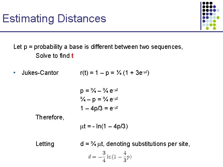
Estimating Distances Let p = probability a base is different between two sequences, Solve to find t • Jukes-Cantor r(t) = 1 – p = ¼ (1 + 3 e-mt) p = ¾ – ¾ e-mt ¾ – p = ¾ e-mt 1 – 4 p/3 = e-mt Therefore, mt = - ln(1 – 4 p/3) Letting d = ¾ mt, denoting substitutions per site,

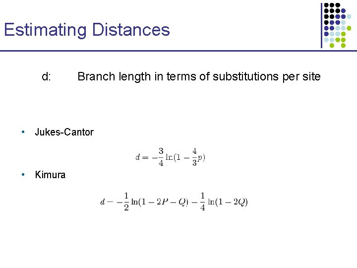
Estimating Distances d: Branch length in terms of substitutions per site • Jukes-Cantor • Kimura

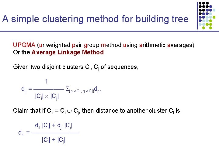
A simple clustering method for building tree UPGMA (unweighted pair group method using arithmetic averages) Or the Average Linkage Method Given two disjoint clusters Ci, Cj of sequences, 1 dij = ––––– {p Ci, q Cj}dpq |Ci| |Cj| Claim that if Ck = Ci Cj, then distance to another cluster Cl is: dil |Ci| + djl |Cj| dkl = ––––––– |Ci| + |Cj|

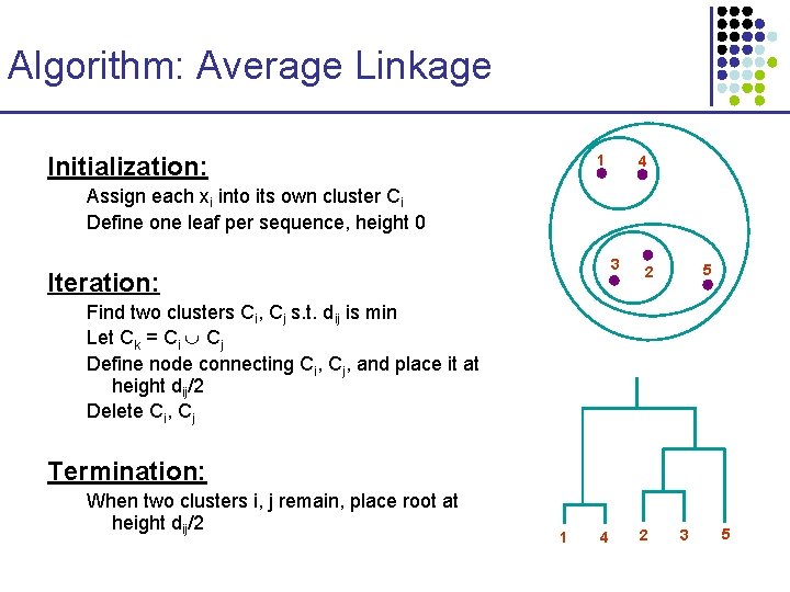
Algorithm: Average Linkage Initialization: 1 4 Assign each xi into its own cluster Ci Define one leaf per sequence, height 0 3 Iteration: 5 2 Find two clusters Ci, Cj s. t. dij is min Let Ck = Ci Cj Define node connecting Ci, Cj, and place it at height dij/2 Delete Ci, Cj Termination: When two clusters i, j remain, place root at height dij/2 1 4 2 3 5

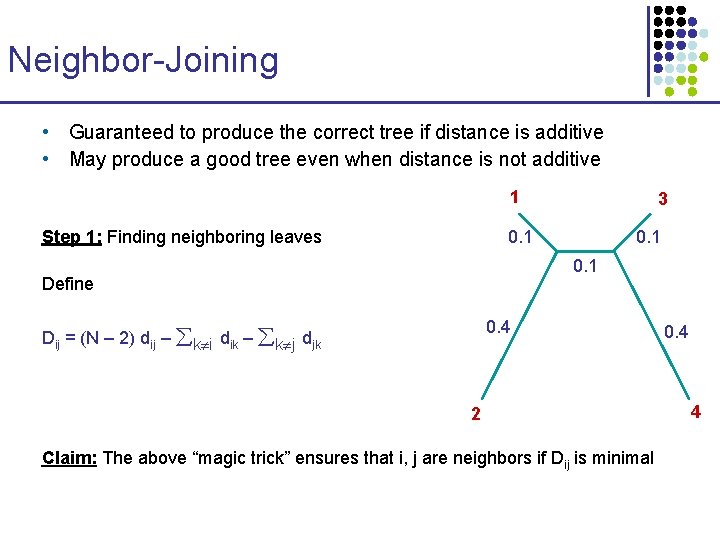
Neighbor-Joining • Guaranteed to produce the correct tree if distance is additive • May produce a good tree even when distance is not additive 1 Step 1: Finding neighboring leaves 3 0. 1 Define 0. 4 Dij = (N – 2) dij – k i dik – k j djk 2 Claim: The above “magic trick” ensures that i, j are neighbors if Dij is minimal 0. 4 4

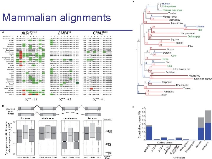
Mammalian alignments

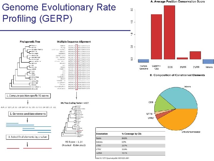
Genome Evolutionary Rate Profiling (GERP)

Species Trees and Gene Trees Rasmussen M D , Kellis M Genome Res. 2007; 17: 1932 -1942 © 2007 by Cold Spring Harbor Laboratory Press

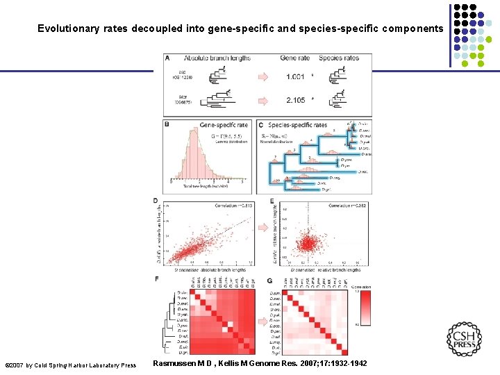
Evolutionary rates decoupled into gene-specific and species-specific components © 2007 by Cold Spring Harbor Laboratory Press Rasmussen M D , Kellis M Genome Res. 2007; 17: 1932 -1942

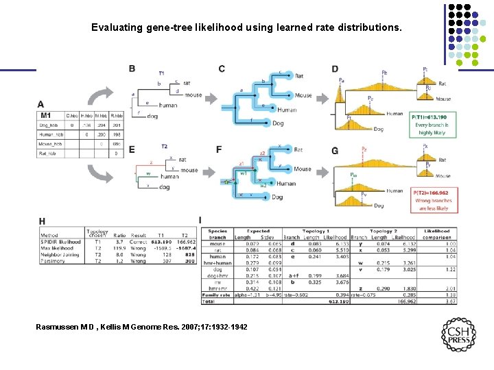
Evaluating gene-tree likelihood using learned rate distributions. Rasmussen M D , Kellis M Genome Res. 2007; 17: 1932 -1942

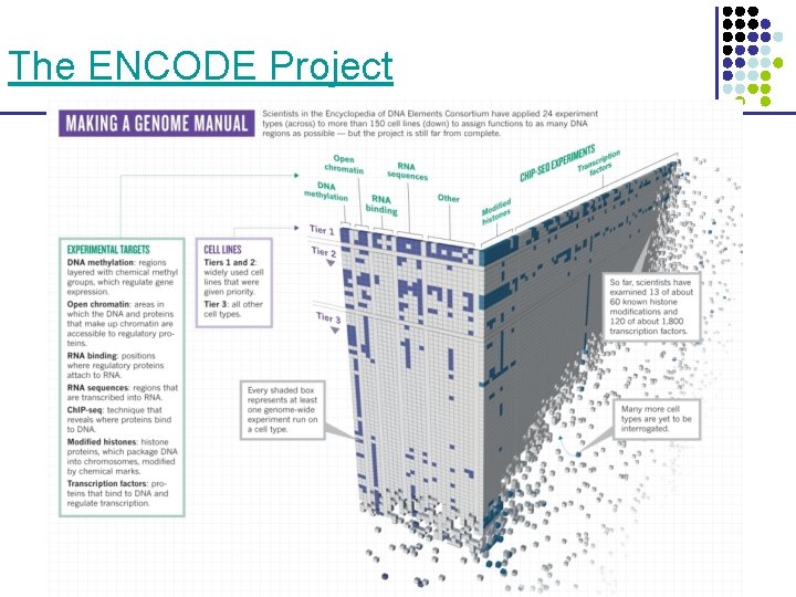
The ENCODE Project

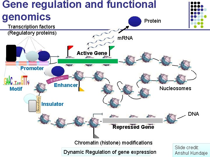
Gene regulation and functional genomics Protein Transcription factors (Regulatory proteins) m. RNA Active Gene Promoter Motif Enhancer Nucleosomes Insulator DNA Repressed Gene Chromatin (histone) modifications Dynamic Regulation of gene expression Slide credit: Anshul Kundaje

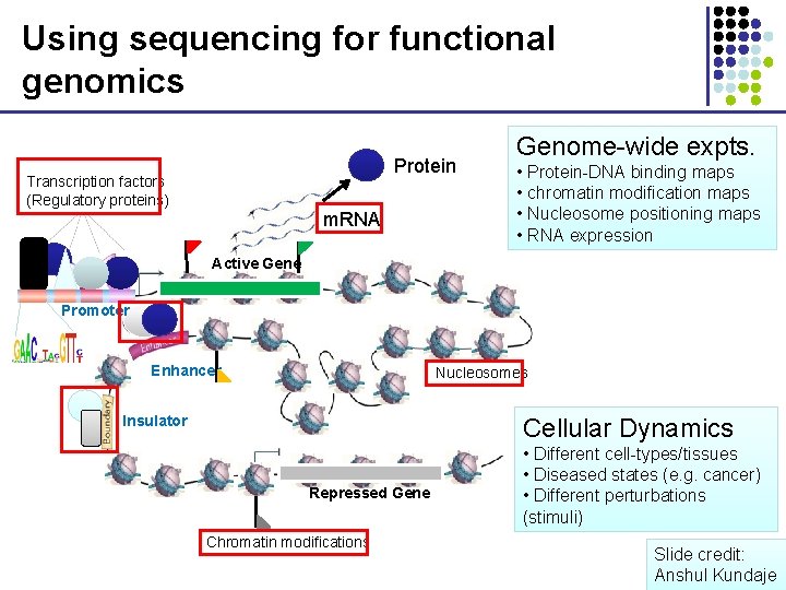
Using sequencing for functional genomics Protein Transcription factors (Regulatory proteins) m. RNA Genome-wide expts. • Protein-DNA binding maps • chromatin modification maps • Nucleosome positioning maps • RNA expression Active Gene Promoter Enhancer Nucleosomes Insulator Cellular Dynamics Repressed Gene Chromatin modifications • Different cell-types/tissues • Diseased states (e. g. cancer) • Different perturbations (stimuli) Slide credit: Anshul Kundaje

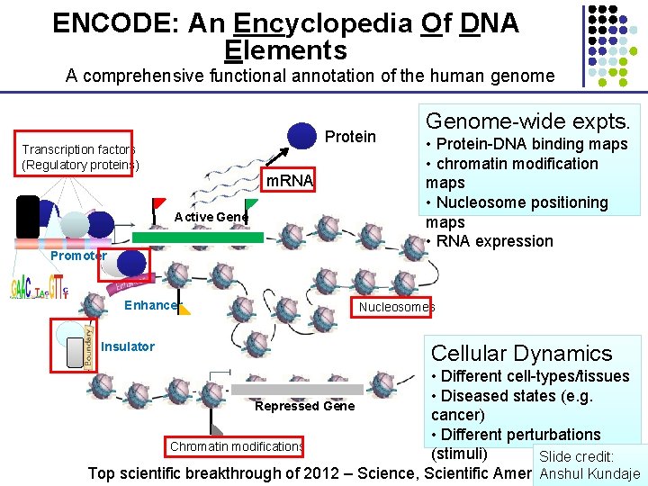
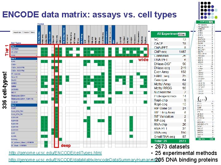
ENCODE: An Encyclopedia Of DNA Elements A comprehensive functional annotation of the human genome Protein Transcription factors (Regulatory proteins) m. RNA Active Gene Promoter Enhancer Insulator Genome-wide expts. • Protein-DNA binding maps • chromatin modification maps • Nucleosome positioning maps • RNA expression Nucleosomes Cellular Dynamics • Different cell-types/tissues • Diseased states (e. g. Repressed Gene cancer) • Different perturbations Chromatin modifications (stimuli) Slide credit: Top scientific breakthrough of 2012 – Science, Scientific American, NIH Anshul Kundaje

Tier 1 ENCODE data matrix: assays vs. cell types 336 cell-types! wide (…) deep • 2673 datasets http: //genome. ucsc. edu/ENCODE/cell. Types. html • 25 experimental methods http: //genome. ucsc. edu/ENCODE/data. Matrix/encode. Data. Summary. Human. html • 205 DNA binding proteins

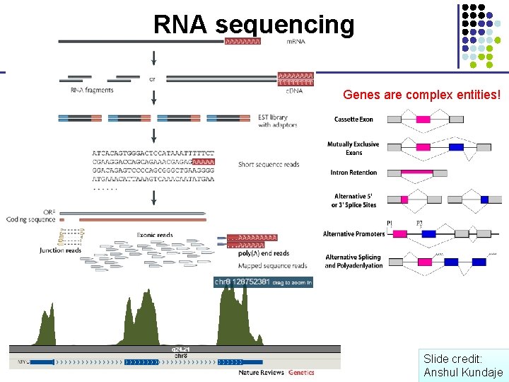
RNA sequencing Genes are complex entities! Slide credit: Anshul Kundaje

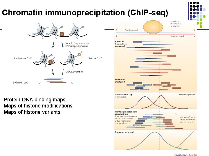
Chromatin immunoprecipitation (Ch. IP-seq) Protein-DNA binding maps Maps of histone modifications Maps of histone variants

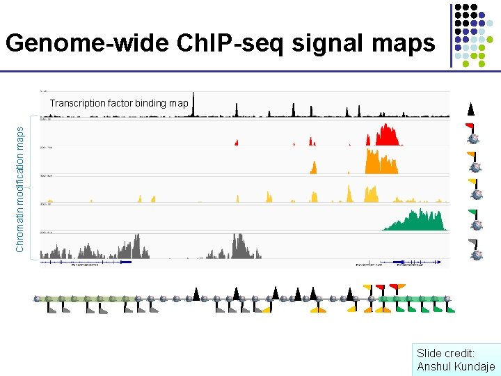
Genome-wide Ch. IP-seq signal maps Chromatin modification maps Transcription factor binding map Slide credit: Anshul Kundaje

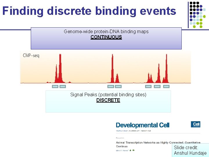
Finding discrete binding events Genome-wide protein-DNA binding maps CONTINUOUS Signal Peaks (potential binding sites) DISCRETE Slide credit: Anshul Kundaje

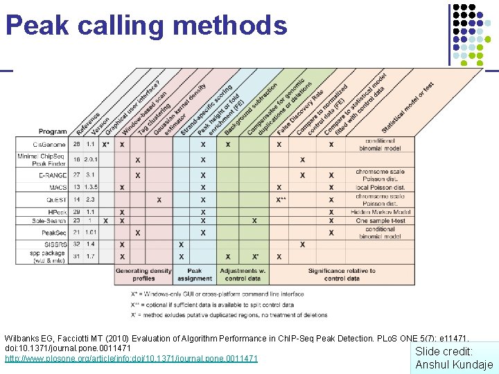
Peak calling methods Wilbanks EG, Facciotti MT (2010) Evaluation of Algorithm Performance in Ch. IP-Seq Peak Detection. PLo. S ONE 5(7): e 11471. doi: 10. 1371/journal. pone. 0011471 Slide credit: http: //www. plosone. org/article/info: doi/10. 1371/journal. pone. 0011471 Anshul Kundaje

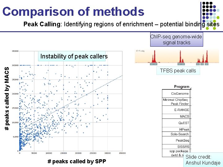
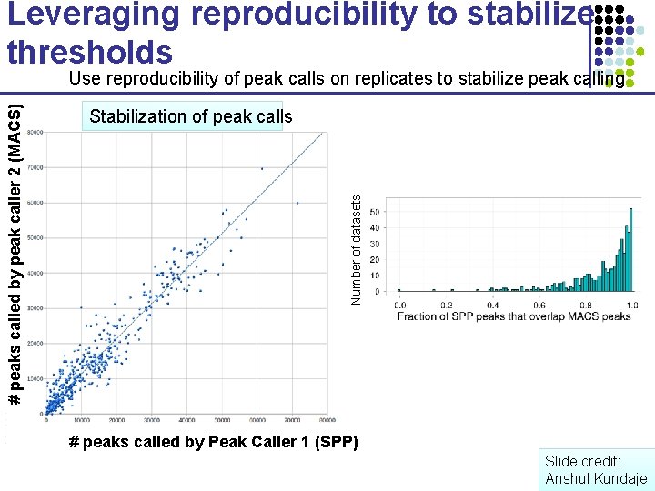
Comparison of methods Peak Calling: Identifying regions of enrichment – potential binding sites Ch. IP-seq genome-wide signal tracks # peaks called by MACS Instability of peak callers TFBS peak calls Challenge: • 1000 s of datasets • Span of 4 years • Different labs and protocols • Different peak callers • Different types of proteins and antibody specificities # peaks called by SPP Slide credit: Anshul Kundaje

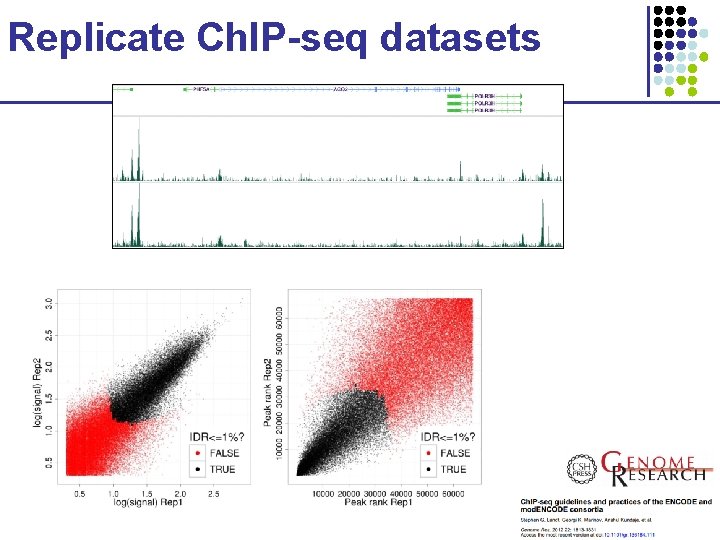
Replicate Ch. IP-seq datasets

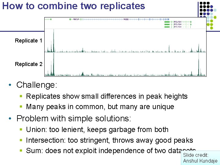
How to combine two replicates Replicate 1 Replicate 2 • Challenge: § Replicates show small differences in peak heights § Many peaks in common, but many are unique • Problem with simple solutions: § Union: too lenient, keeps garbage from both § Intersection: too stringent, throws away good peaks § Sum: does not exploit independence of two datasets Slide credit: Anshul Kundaje

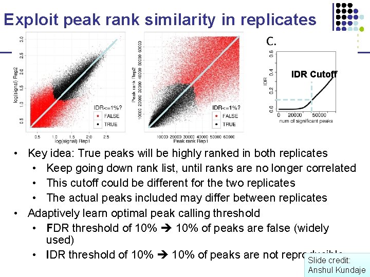
Exploit peak rank similarity in replicates IDR Cutoff • Key idea: True peaks will be highly ranked in both replicates • Keep going down rank list, until ranks are no longer correlated • This cutoff could be different for the two replicates • The actual peaks included may differ between replicates • Adaptively learn optimal peak calling threshold • FDR threshold of 10% of peaks are false (widely used) • IDR threshold of 10% of peaks are not reproducible Slide credit: Anshul Kundaje

Leveraging reproducibility to stabilize thresholds Stabilization of peak calls Number of datasets # peaks called by peak caller 2 (MACS) Use reproducibility of peak calls on replicates to stabilize peak calling # peaks called by Peak Caller 1 (SPP) Slide credit: Anshul Kundaje

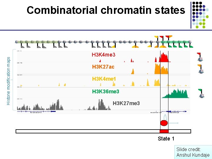
Histone modification maps Combinatorial chromatin states H 3 K 4 me 3 H 3 K 27 ac H 3 K 4 me 1 H 3 K 36 me 3 H 3 K 27 me 3 State 1 Slide credit: Anshul Kundaje

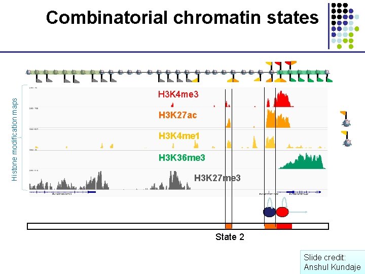
Histone modification maps Combinatorial chromatin states H 3 K 4 me 3 H 3 K 27 ac H 3 K 4 me 1 H 3 K 36 me 3 H 3 K 27 me 3 State 2 Slide credit: Anshul Kundaje

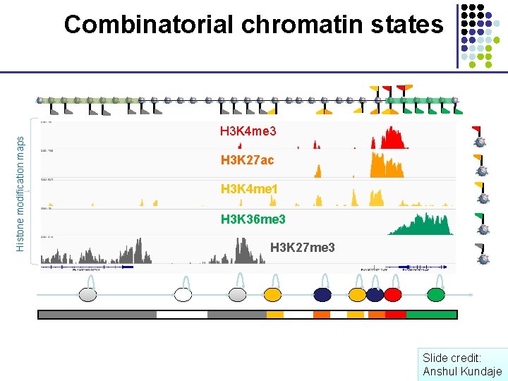
Histone modification maps Combinatorial chromatin states H 3 K 4 me 3 H 3 K 27 ac H 3 K 4 me 1 H 3 K 36 me 3 H 3 K 27 me 3 Slide credit: Anshul Kundaje

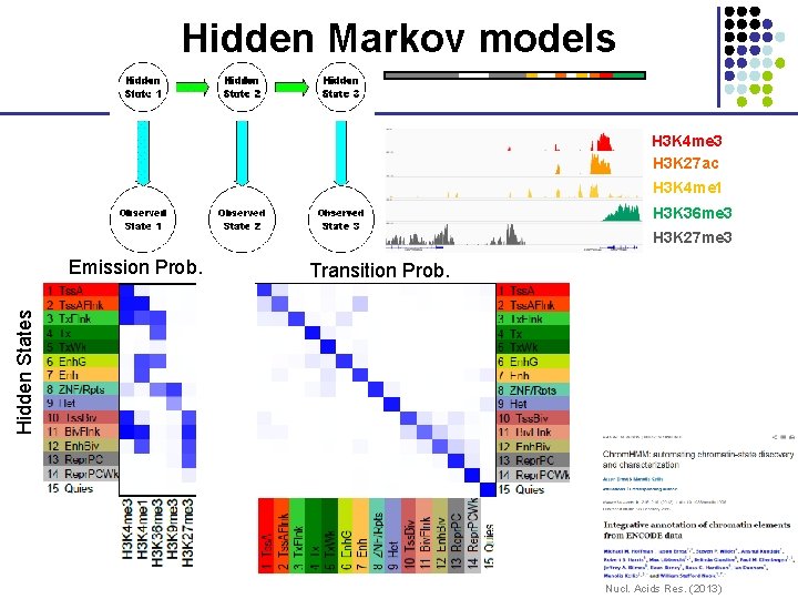
Hidden Markov models H 3 K 4 me 3 H 3 K 27 ac H 3 K 4 me 1 H 3 K 36 me 3 H 3 K 27 me 3 Transition Prob. Hidden States Emission Prob. Nucl. Acids Res. (2013)

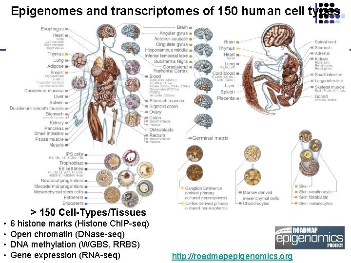
Epigenomes and transcriptomes of 150 human cell types > 150 Cell-Types/Tissues • • 6 histone marks (Histone Ch. IP-seq) Open chromatin (DNase-seq) DNA methylation (WGBS, RRBS) Gene expression (RNA-seq) http: //roadmapepigenomics. org

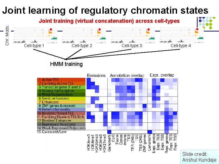
Joint learning of regulatory chromatin states Chr. Mods. Joint training (virtual concatenation) across cell-types Cell-type 1 Cell-type 2 Cell-type 3 Cell-type 4 HMM training Slide credit: Anshul Kundaje

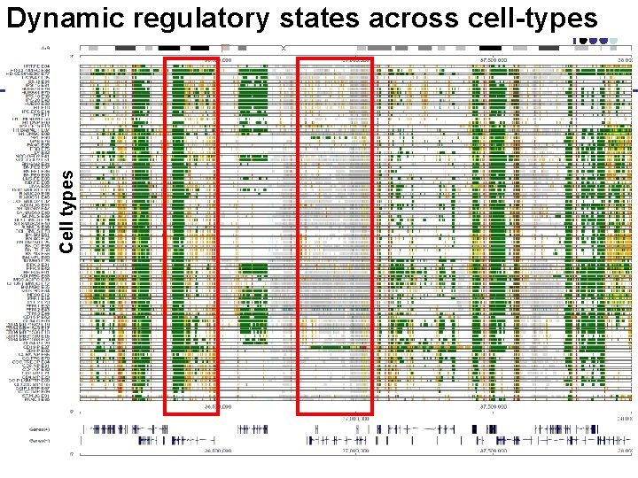
Cell types Dynamic regulatory states across cell-types

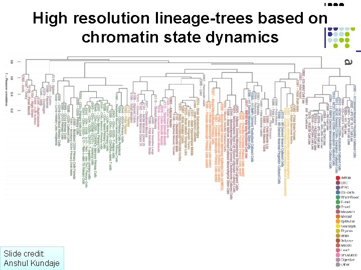
High resolution lineage-trees based on chromatin state dynamics Slide credit: Anshul Kundaje

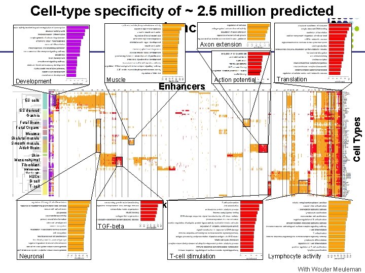
Cell-type specificity of ~ 2. 5 million predicted enhancers Axon extension Development Muscle Enhancers Action potential Translation ES cells Cell Types ES derived Gastric Fetal Brain Fetal Organs Mucosa Skeletal muscle Smooth muscle Adult Brain Skin Mesenchymal Fibroblast Melanocyte Macrophage HSCs B-cell T-cell 500 k Enhancers TGF-beta Neuronal T-cell stimulation Lymphocyte activity With Wouter Meuleman

Sequence Alignment

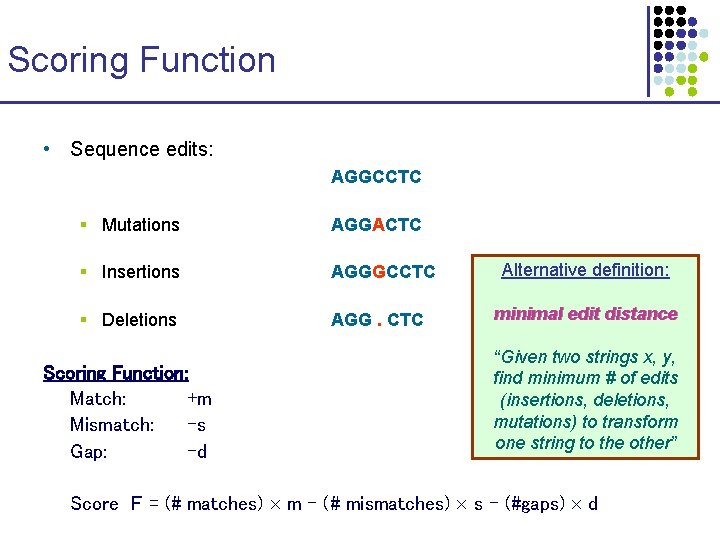
Scoring Function • Sequence edits: AGGCCTC § Mutations AGGACTC § Insertions AGGGCCTC § Deletions AGG. CTC Scoring Function: Match: +m Mismatch: -s Gap: -d Alternative definition: minimal edit distance “Given two strings x, y, find minimum # of edits (insertions, deletions, mutations) to transform one string to the other” Score F = (# matches) m - (# mismatches) s – (#gaps) d

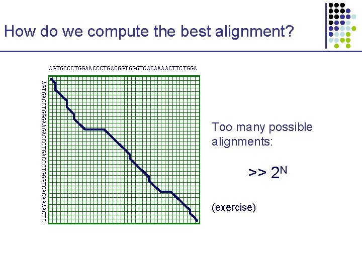
How do we compute the best alignment? AGTGCCCTGGAACCCTGACGGTGGGTCACAAAACTTCTGGA AGTGACCTGGGAAGACCCTGGGTCACAAAACTC Too many possible alignments: >> 2 N (exercise)

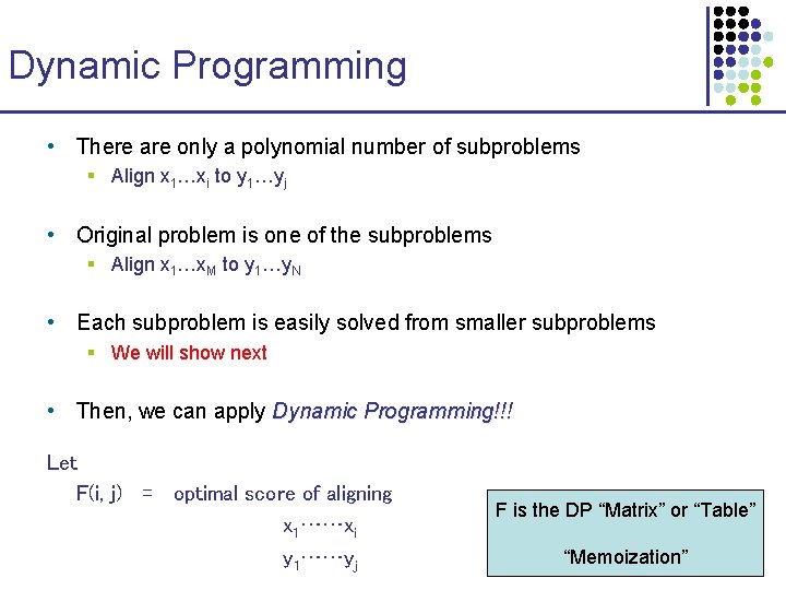
Dynamic Programming • There are only a polynomial number of subproblems § Align x 1…xi to y 1…yj • Original problem is one of the subproblems § Align x 1…x. M to y 1…y. N • Each subproblem is easily solved from smaller subproblems § We will show next • Then, we can apply Dynamic Programming!!! Let F(i, j) = optimal score of aligning x 1……xi y 1……yj F is the DP “Matrix” or “Table” “Memoization”

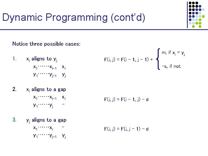
Dynamic Programming (cont’d) Notice three possible cases: 1. 2. 3. xi aligns to yj x 1……xi-1 xi y 1……yj-1 yj m, if xi = yj F(i, j) = F(i – 1, j – 1) + -s, if not xi aligns to a gap x 1……xi-1 xi y 1……yj - F(i, j) = F(i – 1, j) – d yj aligns to a gap x 1……xi y 1……yj-1 yj F(i, j) = F(i, j – 1) – d

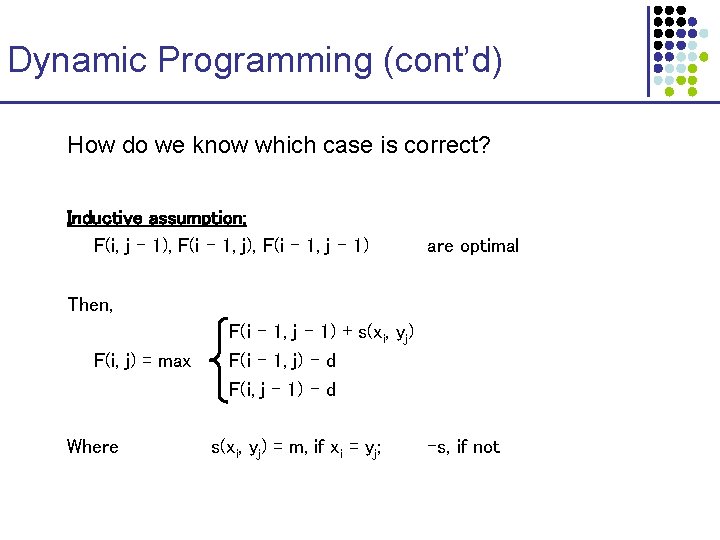
Dynamic Programming (cont’d) How do we know which case is correct? Inductive assumption: F(i, j – 1), F(i – 1, j – 1) are optimal Then, F(i, j) = max Where F(i – 1, j – 1) + s(xi, yj) F(i – 1, j) – d F(i, j – 1) – d s(xi, yj) = m, if xi = yj; -s, if not

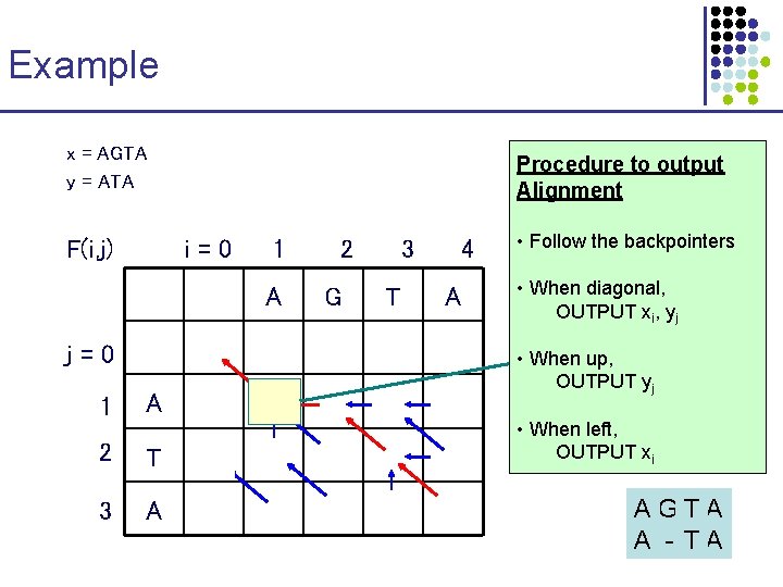
Example x = AGTA y = ATA m= 1 Procedure to output s = -1 Alignment d = -1 F(i, j) i=0 j=0 1 2 3 4 A G T A 0 -1 -2 -3 -4 1 A -1 1 0 -1 -2 2 T -2 0 0 1 0 3 A -3 -1 -1 0 2 • Follow the backpointers F(1, 1) = • When diagonal, + s(A, A), max{F(0, 0) OUTPUT i, y F(0, x 1) –j d, F(1, 0) – d} = • When up, OUTPUT yj max{0 + 1, -1 – 1, • When left, -1 – 1} = 1 OUTPUT xi AGTA A - TA

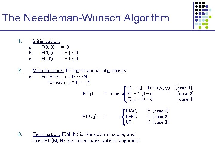
The Needleman-Wunsch Algorithm 1. Initialization. a. b. c. 2. F(0, 0) F(0, j) F(i, 0) = 0 =-j d =-i d Main Iteration. Filling-in partial alignments a. For each i = 1……M For each j = 1……N F(i, j) Ptr(i, j) 3. = max = F(i – 1, j – 1) + s(xi, yj) F(i – 1, j) – d F(i, j – 1) – d DIAG, LEFT, UP, Termination. F(M, N) is the optimal score, and from Ptr(M, N) can trace back optimal alignment if [case 1] if [case 2] if [case 3] [case 1] [case 2] [case 3]

Multiple Sequence Alignments

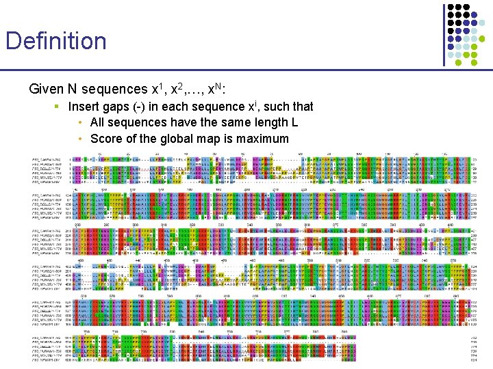
Definition Given N sequences x 1, x 2, …, x. N: § Insert gaps (-) in each sequence xi, such that • All sequences have the same length L • Score of the global map is maximum

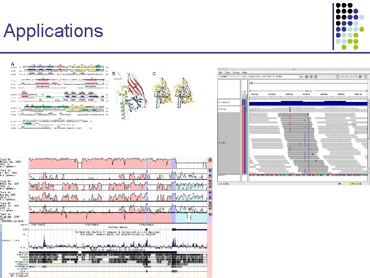
Applications

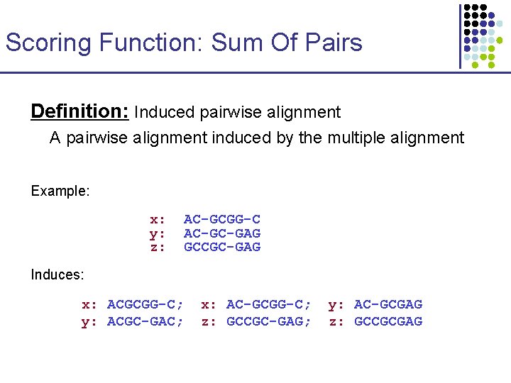
Scoring Function: Sum Of Pairs Definition: Induced pairwise alignment A pairwise alignment induced by the multiple alignment Example: x: y: z: AC-GCGG-C AC-GC-GAG GCCGC-GAG Induces: x: ACGCGG-C; y: ACGC-GAC; x: AC-GCGG-C; z: GCCGC-GAG; y: AC-GCGAG z: GCCGCGAG

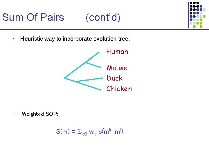
Sum Of Pairs (cont’d) • Heuristic way to incorporate evolution tree: Human Mouse Duck Chicken • Weighted SOP: S(m) = k<l wkl s(mk, ml)

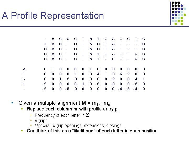
A Profile Representation A C G T - T C C C A A A G G G – – C C C T T T A A A T C C T T 0. 6 0. 2. 2 1 0 0 0 0 1. 2 0 0 0. 8 0 1 0 0. 4 0 0 0. 6 0 0 C C C A A G C C – – T G G G G 0. 8 0 0 0 1 0. 6. 2 0 0. 4 0 0. 2 0 0. 4. 8. 4 0 0 1 0 0 • Given a multiple alignment M = m 1…mn § Replace each column mi with profile entry pi • Frequency of each letter in • # gaps • Optional: # gap openings, extensions, closings § Can think of this as a “likelihood” of each letter in each position

Multiple Sequence Alignments Algorithms

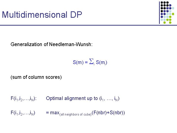
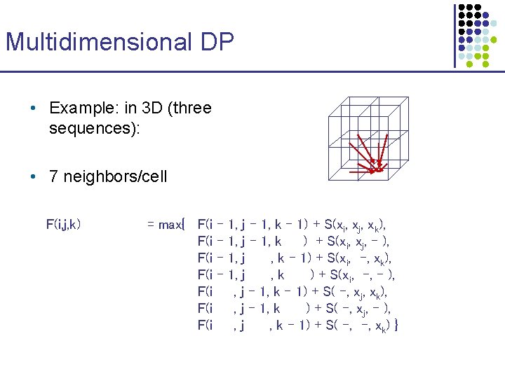
Multidimensional DP Generalization of Needleman-Wunsh: S(m) = i S(mi) (sum of column scores) F(i 1, i 2, …, i. N): Optimal alignment up to (i 1, …, i. N) F(i 1, i 2, …, i. N) = max(all neighbors of cube)(F(nbr)+S(nbr))

Multidimensional DP • Example: in 3 D (three sequences): • 7 neighbors/cell F(i, j, k) = max{ F(i F(i – – 1, j – 1, k – 1) + S(xi, xj, xk), 1, j – 1, k ) + S(xi, xj, - ), 1, j , k – 1) + S(xi, -, xk), 1, j , k ) + S(xi, -, - ), , j – 1, k – 1) + S( -, xj, xk), , j – 1, k ) + S( -, xj, - ), , j , k – 1) + S( -, -, xk) }

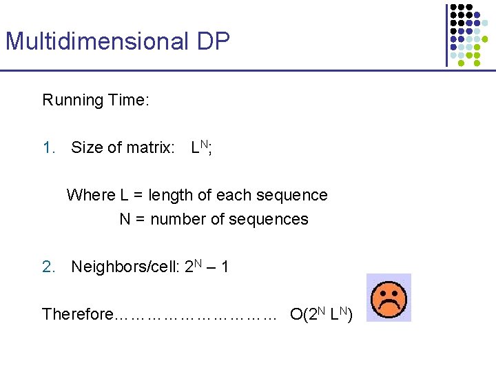
Multidimensional DP Running Time: 1. Size of matrix: LN; Where L = length of each sequence N = number of sequences 2. Neighbors/cell: 2 N – 1 Therefore…………… O(2 N LN)

Multidimensional DP Running Time: 1. Size of matrix: LN; Where L = length of each sequence N = number of sequences 2. Neighbors/cell: 2 N – 1 Therefore…………… O(2 N LN)

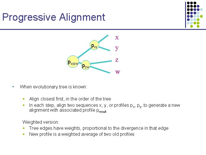
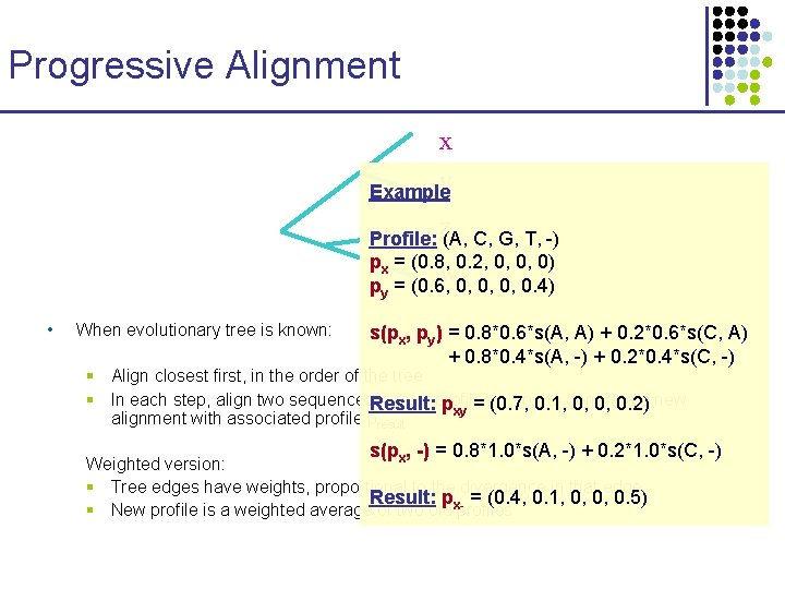
Progressive Alignment x pxyzw • pzw y z w When evolutionary tree is known: § Align closest first, in the order of the tree § In each step, align two sequences x, y, or profiles px, py, to generate a new alignment with associated profile presult Weighted version: § Tree edges have weights, proportional to the divergence in that edge § New profile is a weighted average of two old profiles

Progressive Alignment x y Example z Profile: (A, C, G, T, -) px = (0. 8, 0. 2, 0, 0, 0) w py = (0. 6, 0, 0. 4) • When evolutionary tree is known: s(px, py) = 0. 8*0. 6*s(A, A) + 0. 2*0. 6*s(C, A) + 0. 8*0. 4*s(A, -) + 0. 2*0. 4*s(C, -) § Align closest first, in the order of the tree § In each step, align two sequences. Result: x, y, or profiles px, py 0. 1, , to generate a new pxy = (0. 7, 0, 0, 0. 2) alignment with associated profile presult s(p , -) = 0. 8*1. 0*s(A, -) + 0. 2*1. 0*s(C, -) x Weighted version: § Tree edges have weights, proportional to the divergence in that edge Result: p = (0. 4, 0. 1, 0, 0, 0. 5) § New profile is a weighted average of two old x-profiles

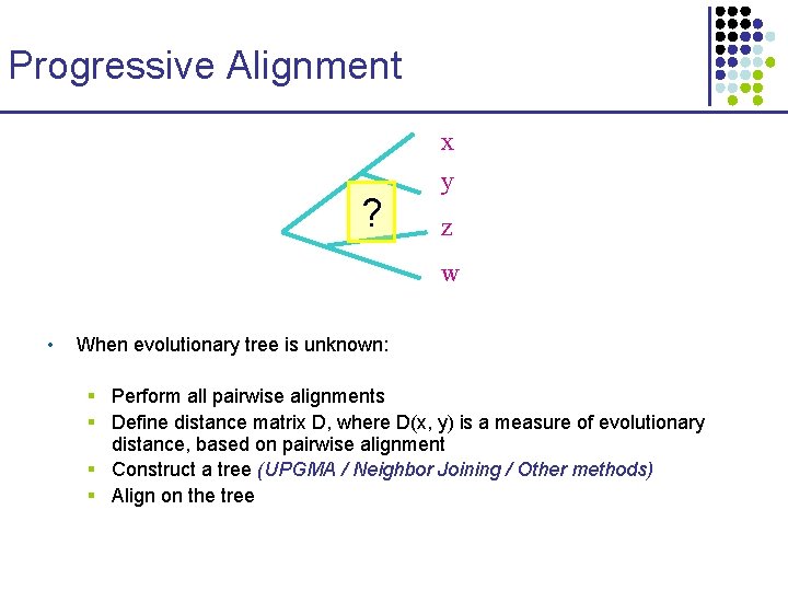
Progressive Alignment x ? y z w • When evolutionary tree is unknown: § Perform all pairwise alignments § Define distance matrix D, where D(x, y) is a measure of evolutionary distance, based on pairwise alignment § Construct a tree (UPGMA / Neighbor Joining / Other methods) § Align on the tree

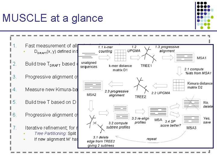
MUSCLE at a glance 1. Fast measurement of all pairwise distances between sequences • DDRAFT(x, y) defined in terms of # common k-mers (k~3) – O(N 2 L log. L) time 2. Build tree TDRAFT based on those distances, with UPGMA 3. Progressive alignment over TDRAFT, resulting in multiple alignment MDRAFT 4. Measure new Kimura-based distances D(x, y) based on MDRAFT 5. Build tree T based on D 6. Progressive alignment over T, to build M 7. Iterative refinement; for many rounds, do: • • Tree Partitioning: Split M on one branch and realign the two resulting profiles If new alignment M’ has better sum-of-pairs score than previous one, accept