Multiple Regression Simple Regression in detail Yi o

Multiple Regression

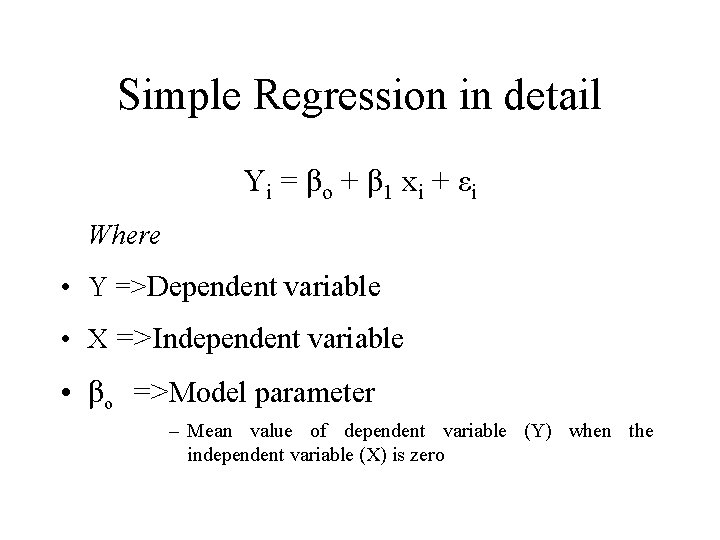
Simple Regression in detail Yi = βo + β 1 xi + εi Where • Y =>Dependent variable • X =>Independent variable • βo =>Model parameter – Mean value of dependent variable (Y) when the independent variable (X) is zero

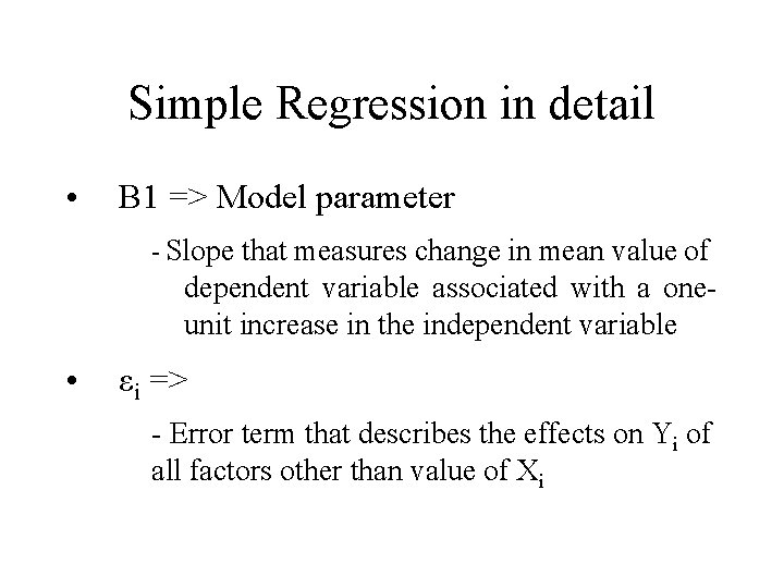
Simple Regression in detail • Β 1 => Model parameter - Slope that measures change in mean value of dependent variable associated with a oneunit increase in the independent variable • εi => - Error term that describes the effects on Yi of all factors other than value of Xi

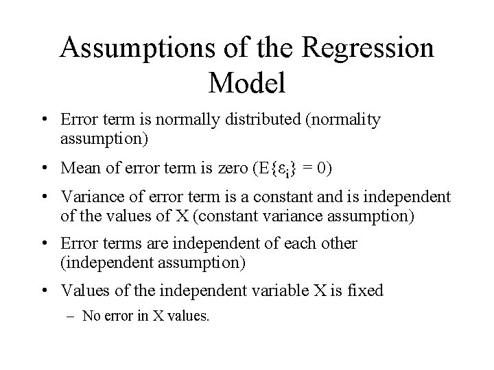
Assumptions of the Regression Model • Error term is normally distributed (normality assumption) • Mean of error term is zero (E{εi} = 0) • Variance of error term is a constant and is independent of the values of X (constant variance assumption) • Error terms are independent of each other (independent assumption) • Values of the independent variable X is fixed – No error in X values.

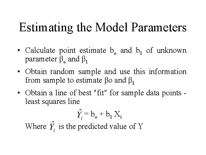
Estimating the Model Parameters • Calculate point estimate bo and b 1 of unknown parameter βo and β 1 • Obtain random sample and use this information from sample to estimate βo and β 1 • Obtain a line of best "fit" for sample data points least squares line = bo + b 1 Xi Where is the predicted value of Y

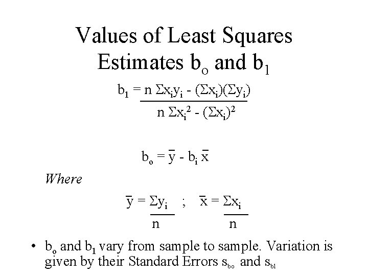
Values of Least Squares Estimates bo and b 1 = n xiyi - ( xi)( yi) n xi 2 - ( xi)2 bo = y - bi x Where y = yi n ; x = xi n • bo and b 1 vary from sample to sample. Variation is given by their Standard Errors Sbo and Sb 1

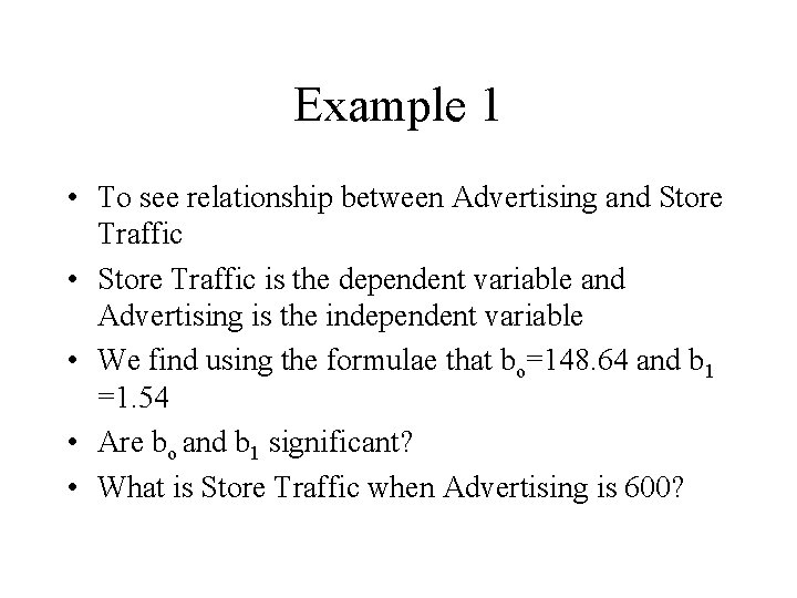
Example 1 • To see relationship between Advertising and Store Traffic • Store Traffic is the dependent variable and Advertising is the independent variable • We find using the formulae that bo=148. 64 and b 1 =1. 54 • Are bo and b 1 significant? • What is Store Traffic when Advertising is 600?

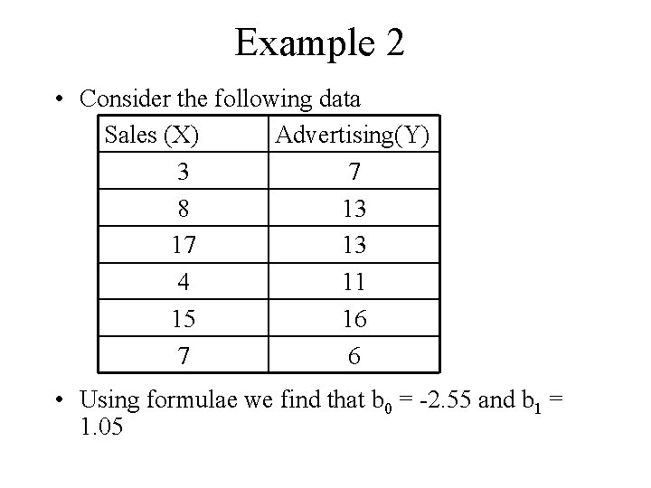
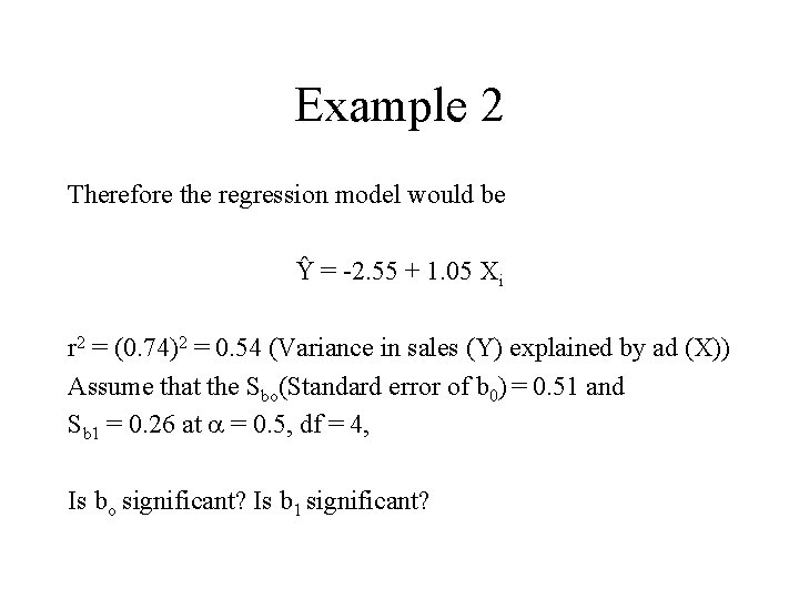
Example 2 • Consider the following data Sales (X) Advertising(Y) 3 7 8 13 17 13 4 11 15 16 7 6 • Using formulae we find that b 0 = -2. 55 and b 1 = 1. 05

Example 2 Therefore the regression model would be Ŷ = -2. 55 + 1. 05 Xi r 2 = (0. 74)2 = 0. 54 (Variance in sales (Y) explained by ad (X)) Assume that the Sbo(Standard error of b 0) = 0. 51 and Sb 1 = 0. 26 at = 0. 5, df = 4, Is bo significant? Is b 1 significant?

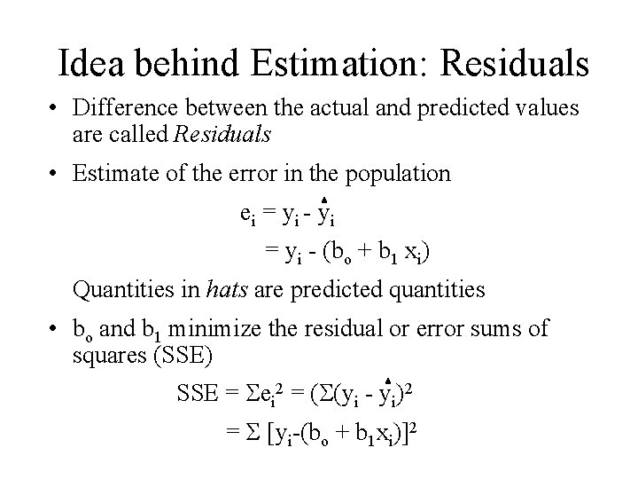
Idea behind Estimation: Residuals • Difference between the actual and predicted values are called Residuals • Estimate of the error in the population ei = yi - yi = yi - (bo + b 1 xi) Quantities in hats are predicted quantities • bo and b 1 minimize the residual or error sums of squares (SSE) SSE = ei 2 = ( (yi - yi)2 = Σ [yi-(bo + b 1 xi)]2

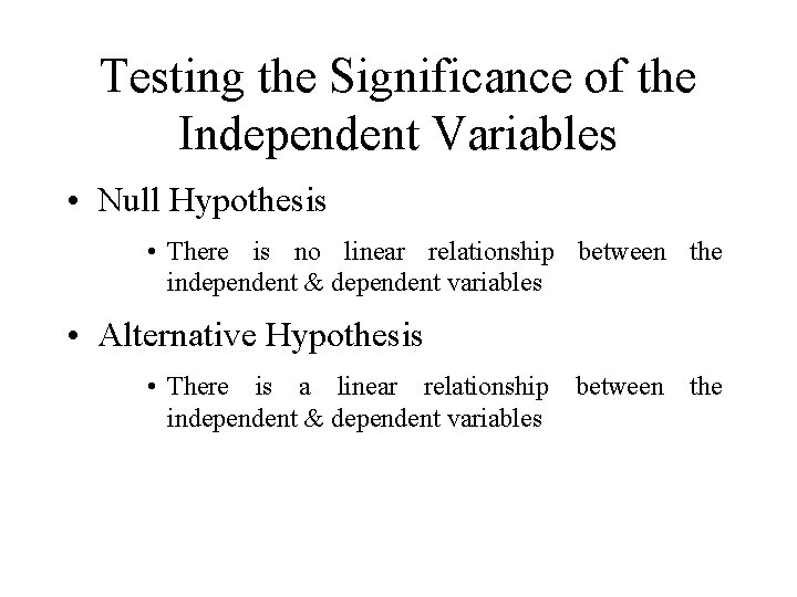
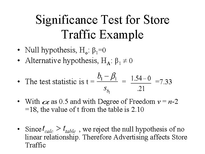
Testing the Significance of the Independent Variables • Null Hypothesis • There is no linear relationship between the independent & dependent variables • Alternative Hypothesis • There is a linear relationship between the independent & dependent variables

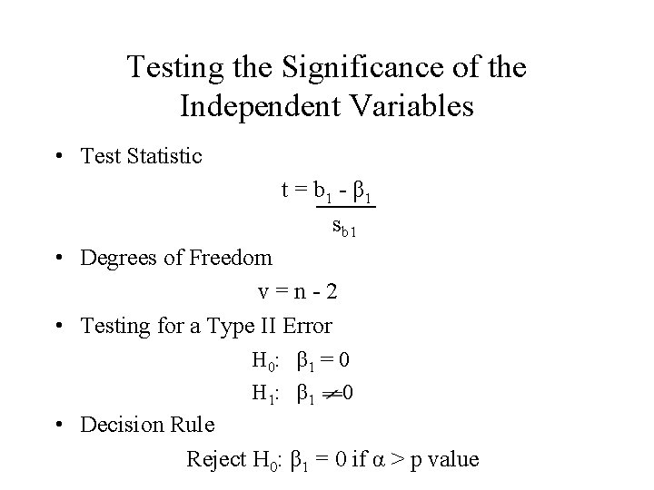
Testing the Significance of the Independent Variables • Test Statistic t = b 1 - β 1 sb 1 • Degrees of Freedom v=n-2 • Testing for a Type II Error H 0: β 1 = 0 H 1: β 1 0 • Decision Rule Reject H 0: β 1 = 0 if α > p value

Significance Test for Store Traffic Example • Null hypothesis, Ho: β 1=0 • Alternative hypothesis, HA: β 1 0 • The test statistic is t = = =7. 33 • With as 0. 5 and with Degree of Freedom v = n-2 =18, the value of t from the table is 2. 10 • Since , we reject the null hypothesis of no linear relationship. Therefore Advertising affects Store Traffic

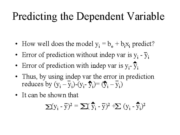
Predicting the Dependent Variable • How well does the model yi = bo + bixi predict? • Error of prediction without indep var is yi - yi • Error of prediction with indep var is yi- yi • Thus, by using indep var the error in prediction reduces by (yi – yi)-(yi- yi)= (yi – yi) • It can be shown that (yi - y)2 = ( yi - y)2 + (yi - yi)2

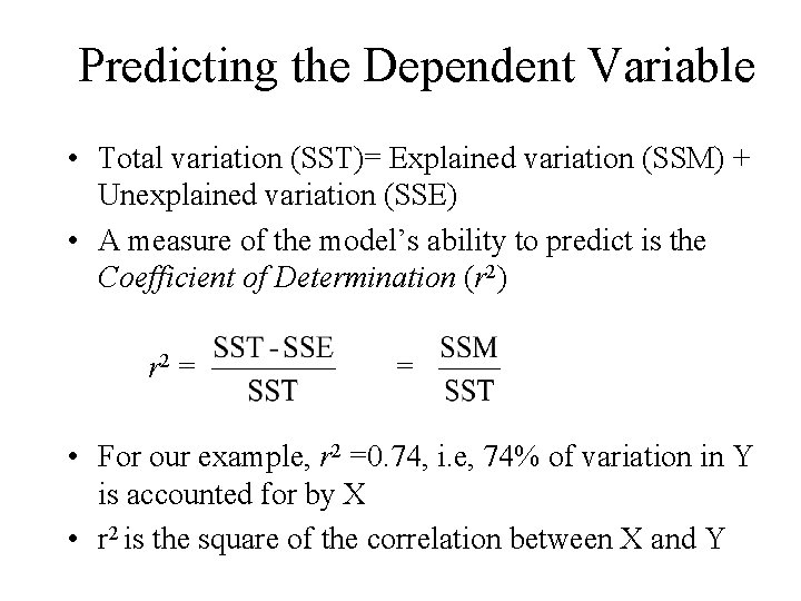
Predicting the Dependent Variable • Total variation (SST)= Explained variation (SSM) + Unexplained variation (SSE) • A measure of the model’s ability to predict is the Coefficient of Determination (r 2) r 2 = = • For our example, r 2 =0. 74, i. e, 74% of variation in Y is accounted for by X • r 2 is the square of the correlation between X and Y

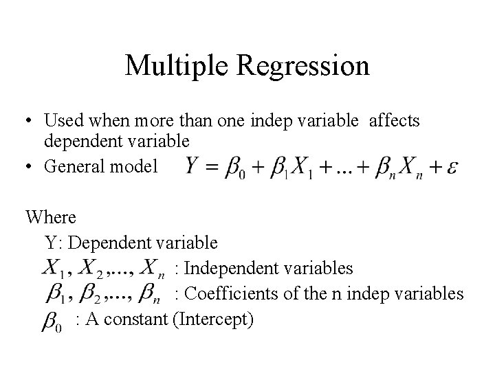
Multiple Regression • Used when more than one indep variable affects dependent variable • General model Where Y: Dependent variable : Independent variables : Coefficients of the n indep variables : A constant (Intercept)

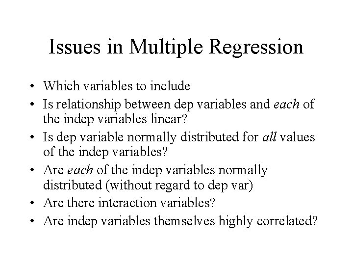
Issues in Multiple Regression • Which variables to include • Is relationship between dep variables and each of the indep variables linear? • Is dep variable normally distributed for all values of the indep variables? • Are each of the indep variables normally distributed (without regard to dep var) • Are there interaction variables? • Are indep variables themselves highly correlated?

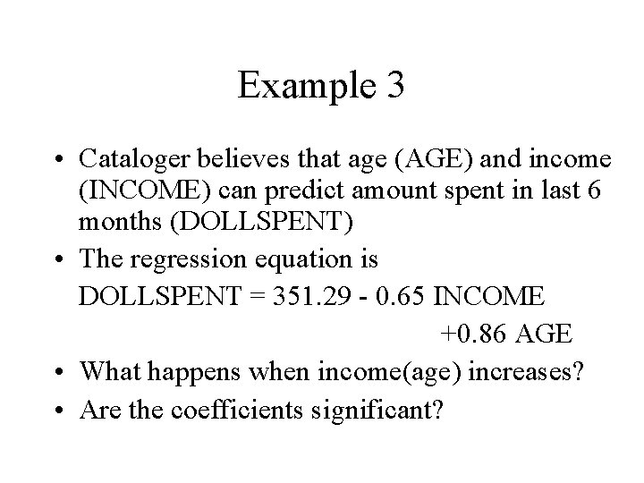
Example 3 • Cataloger believes that age (AGE) and income (INCOME) can predict amount spent in last 6 months (DOLLSPENT) • The regression equation is DOLLSPENT = 351. 29 - 0. 65 INCOME +0. 86 AGE • What happens when income(age) increases? • Are the coefficients significant?

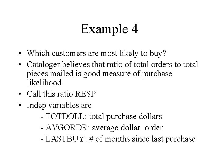
Example 4 • Which customers are most likely to buy? • Cataloger believes that ratio of total orders to total pieces mailed is good measure of purchase likelihood • Call this ratio RESP • Indep variables are - TOTDOLL: total purchase dollars - AVGORDR: average dollar order - LASTBUY: # of months since last purchase

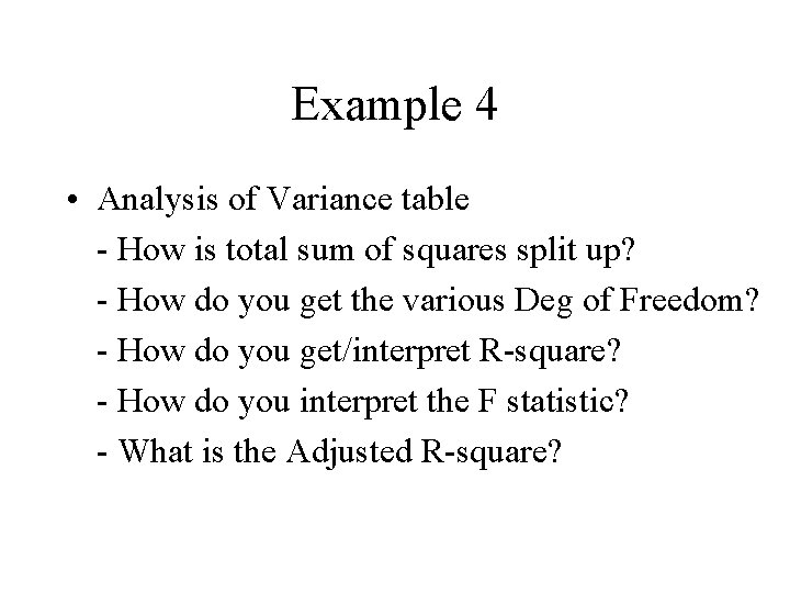
Example 4 • Analysis of Variance table - How is total sum of squares split up? - How do you get the various Deg of Freedom? - How do you get/interpret R-square? - How do you interpret the F statistic? - What is the Adjusted R-square?

Example 4 • Parameter estimates table - What are the t-values corresp to the estimates? - What are the p-values corresp to the estimates? - Which variables are the most important? - What are standardized estimates? - What to do with non-significant variables?