Multiple Regression Models Interactions and Indicator Variables Todays

Multiple Regression Models: Interactions and Indicator Variables

Today’s Data Set ¡ A collector of antique grandfather clocks knows that the price received for the clocks increases linearly with the age of the clocks. Moreover, the collector hypothesizes that the auction price of the clocks will increase linearly as the number of bidders increases. l (Let’s hypothesize a first order MLR model. )

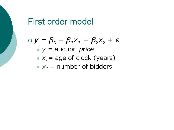
First order model ¡ y = β 0 + β 1 x 1 + β 2 x 2 + ε l l l y = auction price x 1= age of clock (years) x 2 = number of bidders

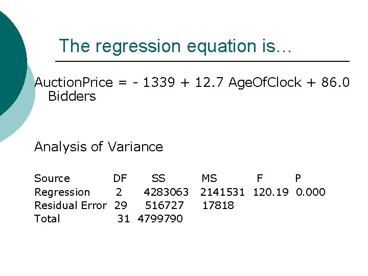
The regression equation is… Auction. Price = - 1339 + 12. 7 Age. Of. Clock + 86. 0 Bidders Analysis of Variance Source DF SS Regression 2 4283063 Residual Error 29 516727 Total 31 4799790 MS F P 2141531 120. 19 0. 000 17818

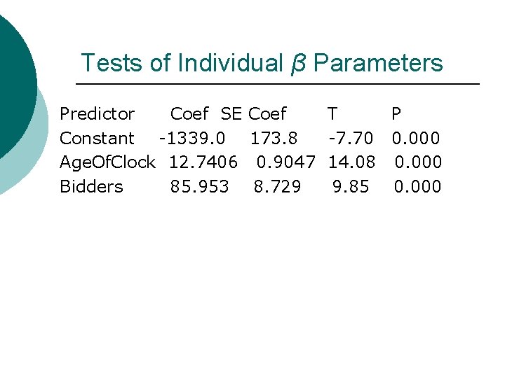
Tests of Individual β Parameters Predictor Coef SE Constant -1339. 0 Age. Of. Clock 12. 7406 Bidders 85. 953 Coef 173. 8 0. 9047 8. 729 T P -7. 70 0. 000 14. 08 0. 000 9. 85 0. 000

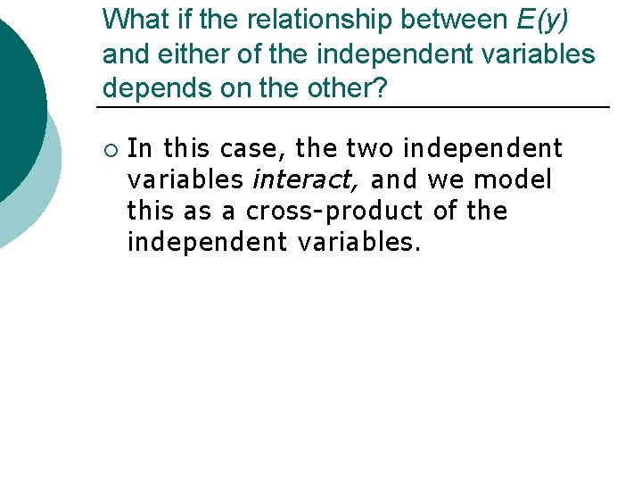
What if the relationship between E(y) and either of the independent variables depends on the other? ¡ In this case, the two independent variables interact, and we model this as a cross-product of the independent variables.

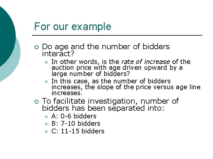
For our example ¡ Do age and the number of bidders interact? l l ¡ In other words, is the rate of increase of the auction price with age driven upward by a large number of bidders? In this case, as the number of bidders increases, the slope of the price versus age line increases. To facilitate investigation, number of bidders has been separated into: l l l A: 0 -6 bidders B: 7 -10 bidders C: 11 -15 bidders

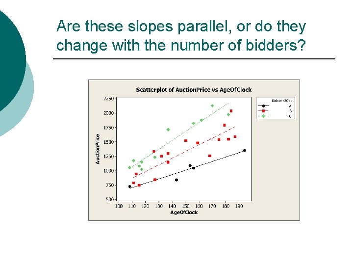
Are these slopes parallel, or do they change with the number of bidders?

Caution! ¡ Once an interaction has been deemed important in a model, all associated first-order terms should be kept in the model, regardless of the magnitude of their p-values.

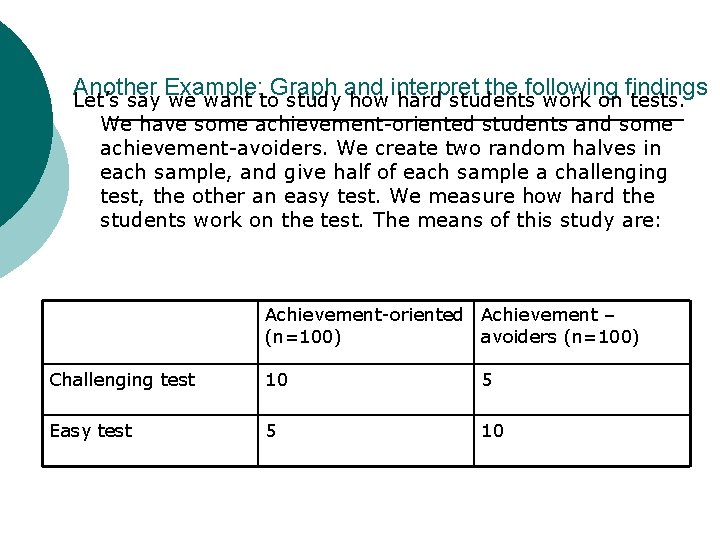
Another Example: Graph and interpret the following findings Let’s say we want to study how hard students work on tests. We have some achievement-oriented students and some achievement-avoiders. We create two random halves in each sample, and give half of each sample a challenging test, the other an easy test. We measure how hard the students work on the test. The means of this study are: Achievement-oriented Achievement – (n=100) avoiders (n=100) Challenging test 10 5 Easy test 5 10

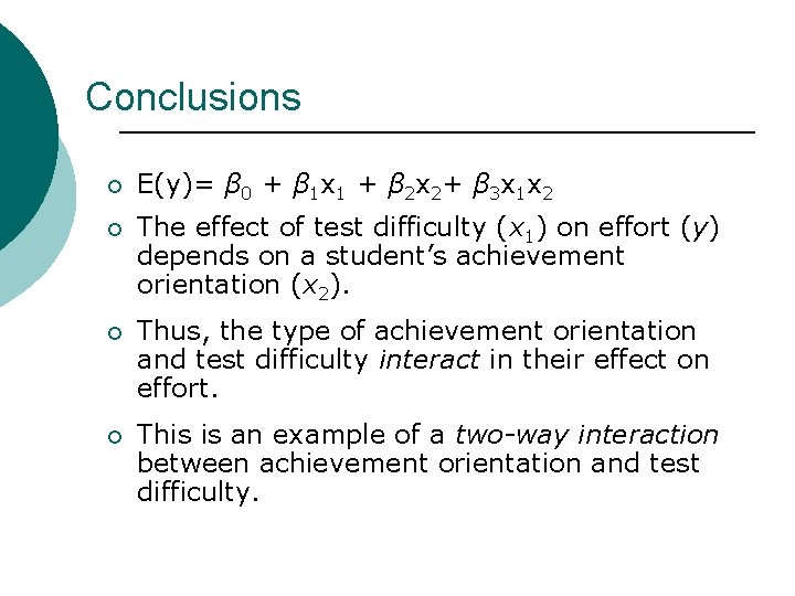
Conclusions ¡ E(y)= β 0 + β 1 x 1 + β 2 x 2+ β 3 x 1 x 2 ¡ The effect of test difficulty (x 1) on effort (y) depends on a student’s achievement orientation (x 2). ¡ Thus, the type of achievement orientation and test difficulty interact in their effect on effort. ¡ This is an example of a two-way interaction between achievement orientation and test difficulty.

Basic premises up to this point ¡ We have used continuous variables (we can assume that having a value of 2 on a variable means having twice as much of it as a 1. ) ¡ We often work with categorical variables in which the different values have no real numerical relationship with each other (race, political affiliation, sex, marital status…) l l ¡ Democrat(1), Independent(2), Republican(3) Is a Republican three times as politically affiliated as a Democrat? How do we resolve this problem?

Dummy Variables ¡ A dummy variable is a numerical variable used in regression analysis to represent subgroups of the sample in your study. ¡ Dummy variables have two values: 0, 1 l ¡ "Republican" variable: someone assigned a 1 on this variable is Republican and someone with an 0 is not. They act like 'switches' that turn various parameters on and off in an equation.

Creating Dummy Variables ¡ In Minitab, we can recode the categorical variable into a set of dummy variables, each of which has two levels. ¡ In the regression model, we will use all but one of the original levels. ¡ The level which is not included in the analysis is the category to which all other categories will be compared (base level. ) You decide this. ¡ The coefficient on the variable in your regression will show the effect that being that variable has on your dependent variable.

Returning to the Clocks at Auction Data Set ¡ The collector of antique grandfather clocks knows that the price received for the clocks increases linearly with the age of the clocks and he hypothesized that the auction price of the clocks will increase linearly as the number of bidders increases. But let’s say he doesn’t have the exact number of bidders, only knows if there was a high number of bidders (we’ll say 9 and above) or a low number (below 9. )

Let’s Create a Dummy Variable in Minitab ¡ ¡ We’ll use the Bidders 2 Cat column Calc Make Indicator Variables l In top box, specify that you want to make indicator variables for Bidders 2 Cat l Let’s store results in C 10 - C 11 Once you have created the variables, name columns 10 and 11 Many. Bidders and Few. Bidders Which is which? Why?

Before we run the analysis… ¡ Let’s say we decide to include Many. Bidders (Few. Bidders is the base level. ) ¡ Because Few. Bidders is not included, we can determine if Many. Bidders predicts a different Auction Price than Few. Bidders. ¡ If Many. Bidders is significant in our regression, with a positive β coefficient, we conclude that Many. Bidders has a significant effect on the price of the clocks at auction.

Thinking Through the Variables ¡ ¡ ¡ What is x 1? Let’s hypothesize the model in plain English… just looking at high/low bidders. ) What’s the Null Hypothesis?

Run the Analysis ¡ ¡ Results of the t-test? What would happen if we used Many. Bidders as our base?

Let’s look at your Journal Application ¡ What does it mean to create a dummy variable and when is it appropriate to do this? ¡ What are all the terms in the original model? ¡ This researcher started with a complex model and simplified it. Which model was better? How can we know?

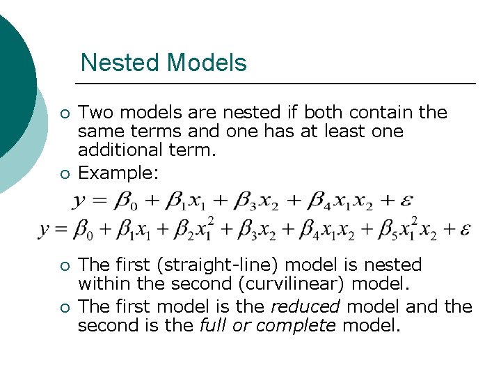
Nested Models ¡ ¡ Two models are nested if both contain the same terms and one has at least one additional term. Example: The first (straight-line) model is nested within the second (curvilinear) model. The first model is the reduced model and the second is the full or complete model.

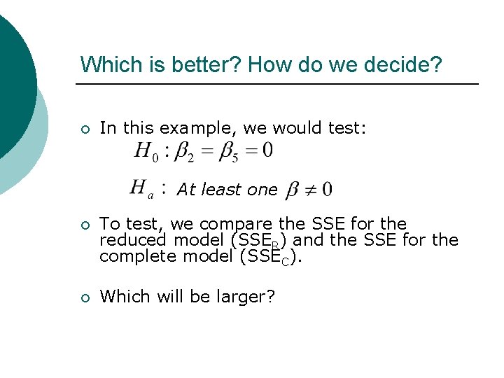
Which is better? How do we decide? ¡ In this example, we would test: At least one ¡ To test, we compare the SSE for the reduced model (SSER) and the SSE for the complete model (SSEC). ¡ Which will be larger?

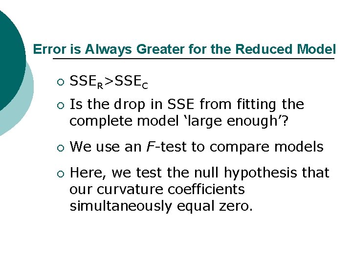
Error is Always Greater for the Reduced Model ¡ ¡ SSER>SSEC Is the drop in SSE from fitting the complete model ‘large enough’? We use an F-test to compare models Here, we test the null hypothesis that our curvature coefficients simultaneously equal zero.

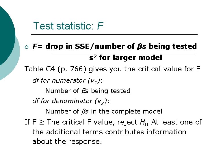
Test statistic: F ¡ F= drop in SSE/number of βs being tested s 2 for larger model Table C 4 (p. 766) gives you the critical value for F df for numerator (v 1): Number of βs being tested df for denominator (v 2): Number of βs in the complete model If F ≥ The critical F value, reject H 0. At least one of the additional terms contributes information about the response.

Conclusions? ¡ Parsimonious models are preferable to big models as long as both have similar predictive power. l ¡ A model is parsimonious when it has a small number of predictors In the end, choice of model is subjective.

Question 3 (Journal) ¡ What type of error do we risk making by conducting multiple ttests? l Pages 184, 188