Multiple Regression Models Advantages of multiple regression Parts

Multiple Regression Models • • Advantages of multiple regression Parts of a multiple regression model & interpretation Raw score vs. Standardized models Differences between r, bbiv, bmult & mult Steps in examining & interpreting a full regression model Underspecification & Proxy Variables Searching for “the model”

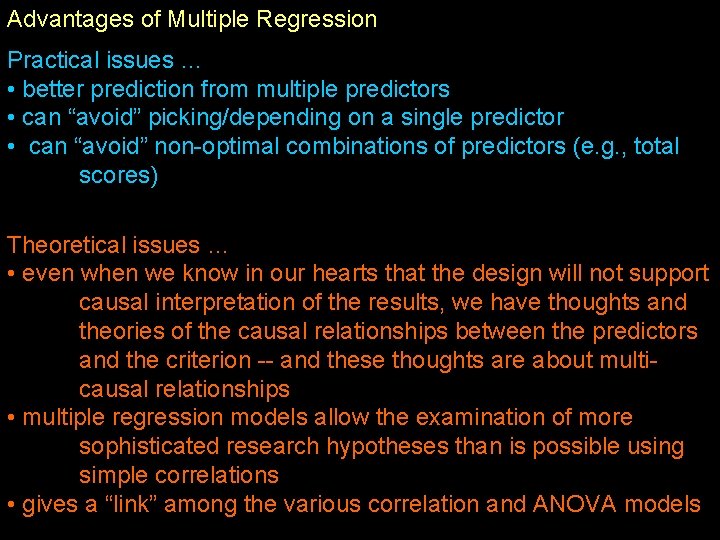
Advantages of Multiple Regression Practical issues … • better prediction from multiple predictors • can “avoid” picking/depending on a single predictor • can “avoid” non-optimal combinations of predictors (e. g. , total scores) Theoretical issues … • even when we know in our hearts that the design will not support causal interpretation of the results, we have thoughts and theories of the causal relationships between the predictors and the criterion -- and these thoughts are about multicausal relationships • multiple regression models allow the examination of more sophisticated research hypotheses than is possible using simple correlations • gives a “link” among the various correlation and ANOVA models

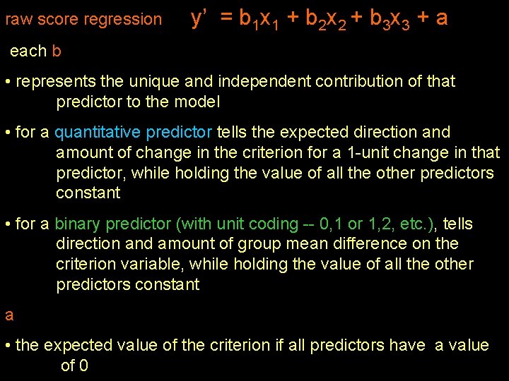
raw score regression y’ = b 1 x 1 + b 2 x 2 + b 3 x 3 + a each b • represents the unique and independent contribution of that predictor to the model • for a quantitative predictor tells the expected direction and amount of change in the criterion for a 1 -unit change in that predictor, while holding the value of all the other predictors constant • for a binary predictor (with unit coding -- 0, 1 or 1, 2, etc. ), tells direction and amount of group mean difference on the criterion variable, while holding the value of all the other predictors constant a • the expected value of the criterion if all predictors have a value of 0

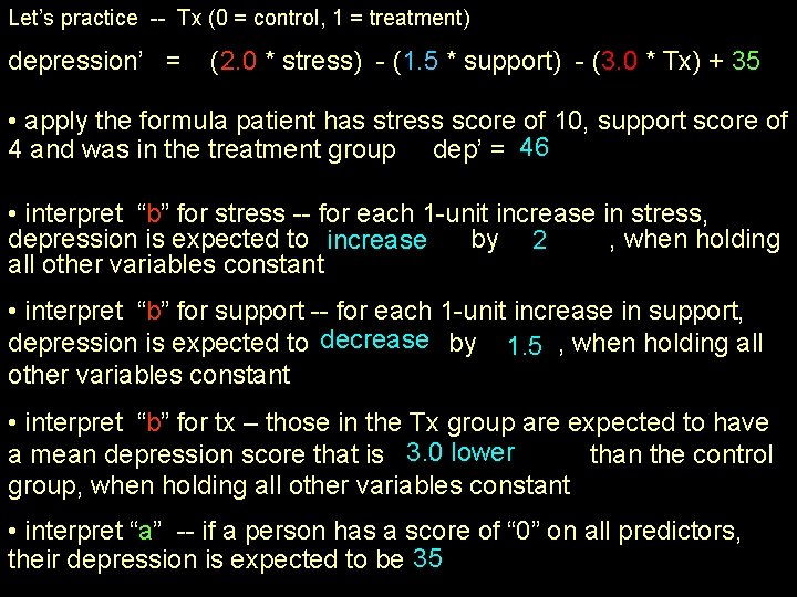
Let’s practice -- Tx (0 = control, 1 = treatment) depression’ = (2. 0 * stress) - (1. 5 * support) - (3. 0 * Tx) + 35 • apply the formula patient has stress score of 10, support score of 4 and was in the treatment group dep’ = 46 • interpret “b” for stress -- for each 1 -unit increase in stress, depression is expected to increase by 2 , when holding all other variables constant • interpret “b” for support -- for each 1 -unit increase in support, depression is expected to decrease by 1. 5 , when holding all other variables constant • interpret “b” for tx – those in the Tx group are expected to have a mean depression score that is 3. 0 lower than the control group, when holding all other variables constant • interpret “a” -- if a person has a score of “ 0” on all predictors, their depression is expected to be 35

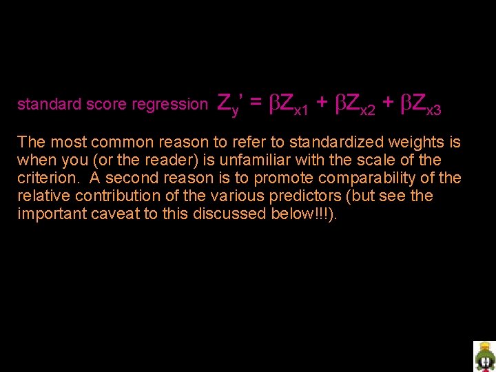
standard score regression Zy’ = Zx 1 + Zx 2 + Zx 3 The most common reason to refer to standardized weights is when you (or the reader) is unfamiliar with the scale of the criterion. A second reason is to promote comparability of the relative contribution of the various predictors (but see the important caveat to this discussed below!!!).

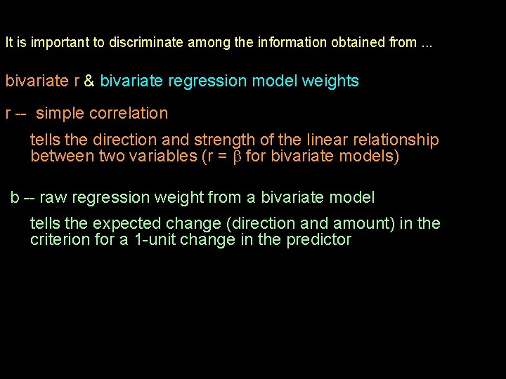
It is important to discriminate among the information obtained from. . . bivariate r & bivariate regression model weights r -- simple correlation tells the direction and strength of the linear relationship between two variables (r = for bivariate models) b -- raw regression weight from a bivariate model tells the expected change (direction and amount) in the criterion for a 1 -unit change in the predictor

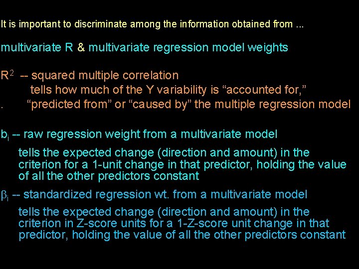
It is important to discriminate among the information obtained from. . . multivariate R & multivariate regression model weights R 2 -- squared multiple correlation tells how much of the Y variability is “accounted for, ”. “predicted from” or “caused by” the multiple regression model bi -- raw regression weight from a multivariate model tells the expected change (direction and amount) in the criterion for a 1 -unit change in that predictor, holding the value of all the other predictors constant i -- standardized regression wt. from a multivariate model tells the expected change (direction and amount) in the criterion in Z-score units for a 1 -Z-score unit change in that predictor, holding the value of all the other predictors constant

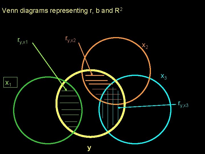
Venn diagrams representing r, b and R 2 ry, x 1 ry, x 2 x 3 x 1 ry, x 3 y

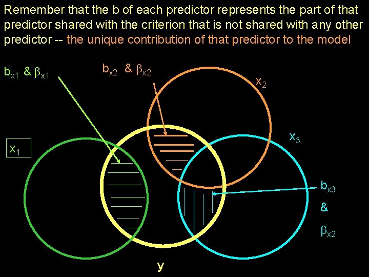
Remember that the b of each predictor represents the part of that predictor shared with the criterion that is not shared with any other predictor -- the unique contribution of that predictor to the model bx 1 & x 1 bx 2 & x 2 x 3 x 1 bx 3 & x 2 y

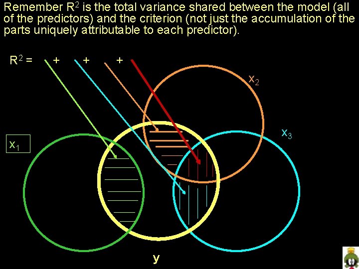
Remember R 2 is the total variance shared between the model (all of the predictors) and the criterion (not just the accumulation of the parts uniquely attributable to each predictor). R 2 = + + + x 2 x 3 x 1 y

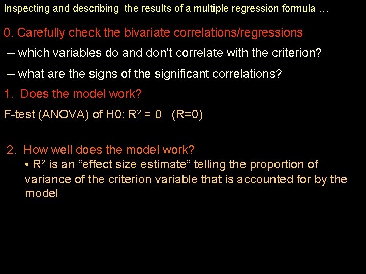
Inspecting and describing the results of a multiple regression formula … 0. Carefully check the bivariate correlations/regressions -- which variables do and don’t correlate with the criterion? -- what are the signs of the significant correlations? 1. Does the model work? F-test (ANOVA) of H 0: R² = 0 (R=0) 2. How well does the model work? • R² is an “effect size estimate” telling the proportion of variance of the criterion variable that is accounted for by the model

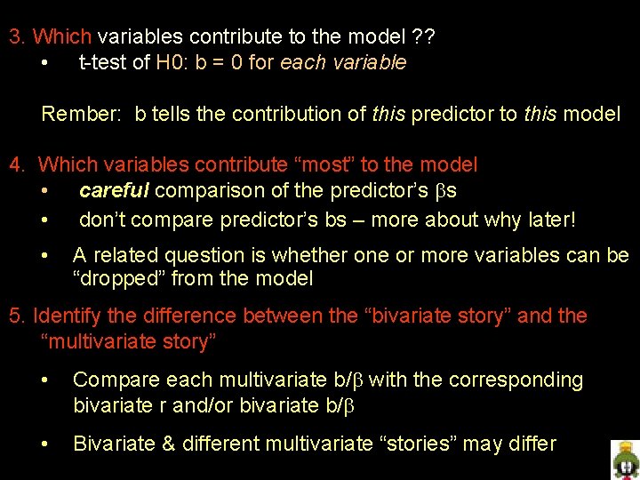
3. Which variables contribute to the model ? ? • t-test of H 0: b = 0 for each variable Rember: b tells the contribution of this predictor to this model 4. Which variables contribute “most” to the model • careful comparison of the predictor’s s • don’t compare predictor’s bs – more about why later! • A related question is whether one or more variables can be “dropped” from the model 5. Identify the difference between the “bivariate story” and the “multivariate story” • Compare each multivariate b/ with the corresponding bivariate r and/or bivariate b/ • Bivariate & different multivariate “stories” may differ

Model Specification & why it matters !!! What we need to remember is that we will never, ever (even once) have a “properly specified” multiple regression model one that includes all of & only the causal variables influencing the criterion ! What can we do about “misspecification” ? • running larger models with every available predictor in them won’t help – models with many predictors tend to get really messy • our best hope is to base our regression models upon the existing literature & good theory and to apply programmatic researc

Proxy variables Remember (again) we are not going to have experimental data! The variables we have might be the actual causal variables influencing this criterion, or (more likely) they might only be correlates of those causal variables – proxy variables Many of the “subject variables” that are very common in multivariate modeling are of this ilk… • is it really “personality, ” “ethnicity”, “age” that are driving the criterion – or is it all the differences in the experiences, opportunities, or other correlates of these variables? • is it really the “number of practices” or the things that, in turn, produced the number of practices that were chosen? Again, replication and convergence (trying alternative measure of the involved constructs) can help decide if our predictors are representing what we think the do!!

Proxy variables In sense, proxy variables are a kind of “confounds” because we are attributing an effect to one variable when it might be due to another. We can take a similar effect to understanding proxys that we do to understanding confounds we have to rule out specific alternative explanations !!! An example r personality, performance =. 4 Is it really personality? Motivation, amount of preparation & testing comfort are some variables that have and are all related to perf. So, we run a multiple regression with all four as predictors. If personality doesn’t contribute, then it isn’t personality but the other variables. If personality contributes to that model, then we know that “personality” in the model is “the part of personality that isn’t motivation, preparation or comfort”.