Multiple Regression Forecasts Materials for this lecture Demo

Multiple Regression Forecasts • Materials for this lecture • Demo Lecture 8 Multiple Regression. XLSX • Read Chapter 15 Pages 8 -9 • Read all of Chapter 16’s Section 13

Black Swans (BSs) -- Taleb • BSs low probability events – An outlier “outside realm of reasonable expectations” – Carries an extreme impact – Human nature causes us to concoct explanations • Black swans are an example of uncertainty – Uncertainty is generated by unknown probability distributions – Risk is generated by “known” distributions • 2008 recession was a BSs – A depression is a BSs – Dramatic increases of grain prices in 2006 and 2007 – Dramatic increase in cotton price in 2010

Fat Tails and Forecasting – Mandelbrot – founder of fractile science observed that financial markets had fatter tails than an normal distribution implies. – Taleb warns that people tend to underestimate risk, especially when armed with statistical models built on normal distributions. – Posner offer this warning: We live in an information rich environment so we must seek out the right balance between human intuition and computer analysis. – These cautions are offered now because we are expected to use a normal distribution to simulate residuals from a multiple regression model.

Structural Variation • Variables you want to forecast are often dependent on other variables Qt. Demand = f( Own Price, Competing Price, Income, Population, Season, Tastes & Preferences, Trend, etc. ) Y = a + b (Time) • Structural models will explain most structural variation in a data series – Even when we build structural models, the forecast is not perfect – A residual remains as the unexplained portion

Structural Variation

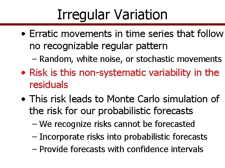
Irregular Variation • Erratic movements in time series that follow no recognizable regular pattern – Random, white noise, or stochastic movements • Risk is this non-systematic variability in the residuals • This risk leads to Monte Carlo simulation of the risk for our probabilistic forecasts – We recognize risks cannot be forecasted – Incorporate risks into probabilistic forecasts – Provide forecasts with confidence intervals

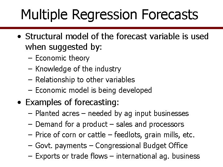
Multiple Regression Forecasts • Structural model of the forecast variable is used when suggested by: – – Economic theory Knowledge of the industry Relationship to other variables Economic model is being developed • Examples of forecasting: – – – Planted acres – needed by ag input businesses Demand for a product – sales and processors Price of corn or cattle – feedlots, grain mills, etc. Govt. payments – Congressional Budget Office Exports or trade flows – international ag. business

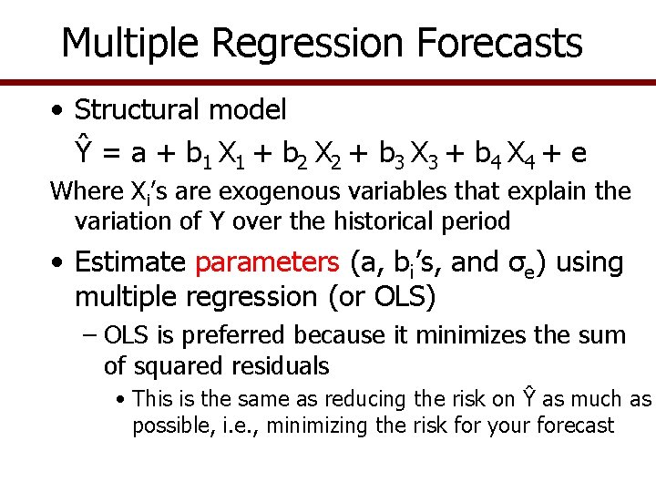
Multiple Regression Forecasts • Structural model Ŷ = a + b 1 X 1 + b 2 X 2 + b 3 X 3 + b 4 X 4 + e Where Xi’s are exogenous variables that explain the variation of Y over the historical period • Estimate parameters (a, bi’s, and σe) using multiple regression (or OLS) – OLS is preferred because it minimizes the sum of squared residuals • This is the same as reducing the risk on Ŷ as much as possible, i. e. , minimizing the risk for your forecast

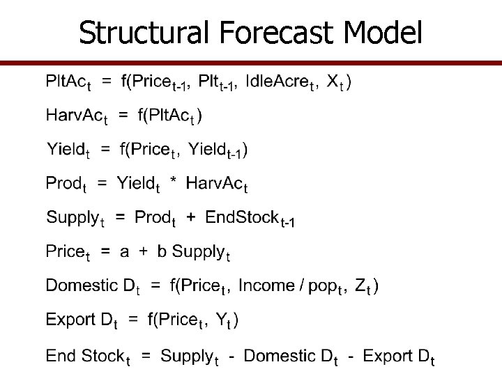
Structural Forecast Model

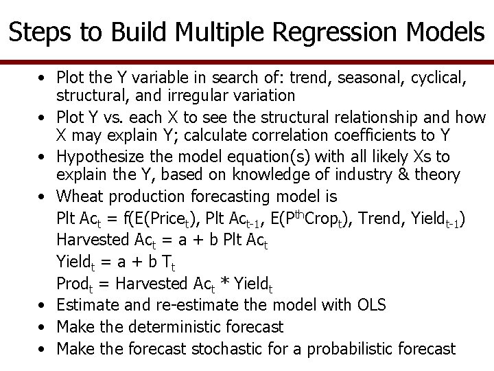
Steps to Build Multiple Regression Models • Plot the Y variable in search of: trend, seasonal, cyclical, structural, and irregular variation • Plot Y vs. each X to see the structural relationship and how X may explain Y; calculate correlation coefficients to Y • Hypothesize the model equation(s) with all likely Xs to explain the Y, based on knowledge of industry & theory • Wheat production forecasting model is Plt Act = f(E(Pricet), Plt Act-1, E(Pth. Cropt), Trend, Yieldt-1) Harvested Act = a + b Plt Act Yieldt = a + b Tt Prodt = Harvested Act * Yieldt • Estimate and re-estimate the model with OLS • Make the deterministic forecast • Make the forecast stochastic for a probabilistic forecast

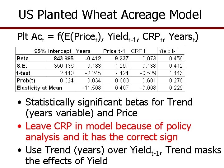
US Planted Wheat Acreage Model Plt Act = f(E(Pricet), Yieldt-1, CRPt, Yearst) • Statistically significant betas for Trend (years variable) and Price • Leave CRP in model because of policy analysis and it has the correct sign • Use Trend (years) over Yieldt-1, Trend masks the effects of Yield

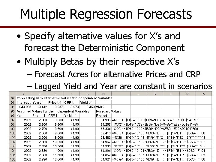
Multiple Regression Forecasts • Specify alternative values for X’s and forecast the Deterministic Component • Multiply Betas by their respective X’s – Forecast Acres for alternative Prices and CRP – Lagged Yield and Year are constant in scenarios

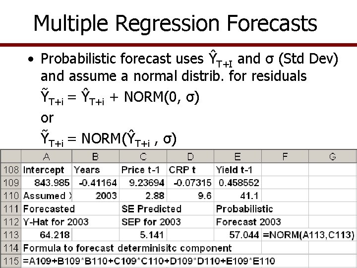
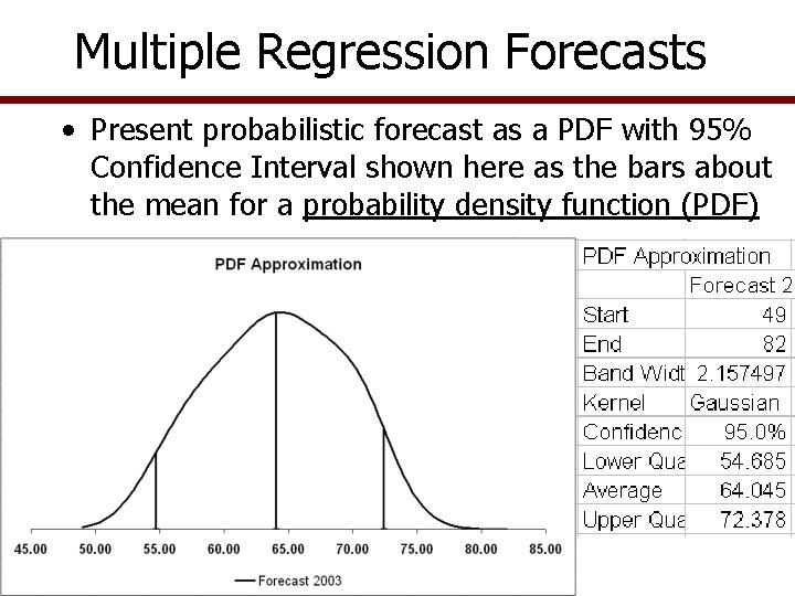
Multiple Regression Forecasts • Probabilistic forecast uses ŶT+I and σ (Std Dev) and assume a normal distrib. for residuals ỸT+i = ŶT+i + NORM(0, σ) or ỸT+i = NORM(ŶT+i , σ)

Multiple Regression Forecasts • Present probabilistic forecast as a PDF with 95% Confidence Interval shown here as the bars about the mean for a probability density function (PDF)

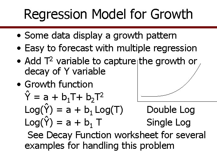
Regression Model for Growth • Some data display a growth pattern • Easy to forecast with multiple regression • Add T 2 variable to capture the growth or decay of Y variable • Growth function Ŷ = a + b 1 T+ b 2 T 2 Log(Ŷ) = a + b 1 Log(T) Double Log(Ŷ) = a + b 1 T Single Log See Decay Function worksheet for several examples for handling this problem

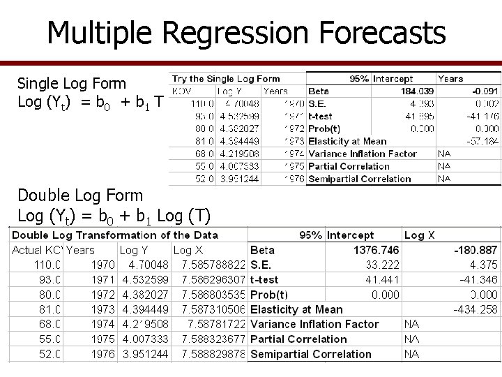
Multiple Regression Forecasts Single Log Form Log (Yt) = b 0 + b 1 T Double Log Form Log (Yt) = b 0 + b 1 Log (T)

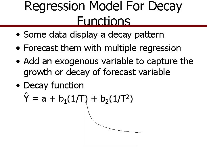
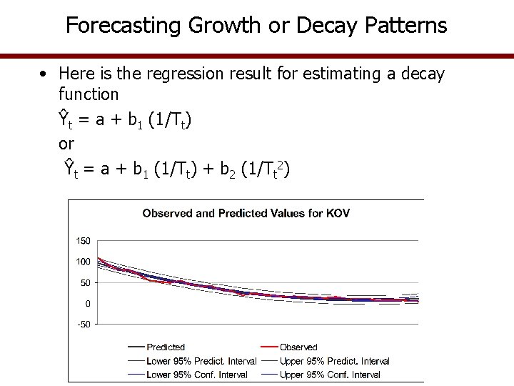
Regression Model For Decay Functions • Some data display a decay pattern • Forecast them with multiple regression • Add an exogenous variable to capture the growth or decay of forecast variable • Decay function Ŷ = a + b 1(1/T) + b 2(1/T 2)

Forecasting Growth or Decay Patterns • Here is the regression result for estimating a decay function Ŷt = a + b 1 (1/Tt) or Ŷt = a + b 1 (1/Tt) + b 2 (1/Tt 2)

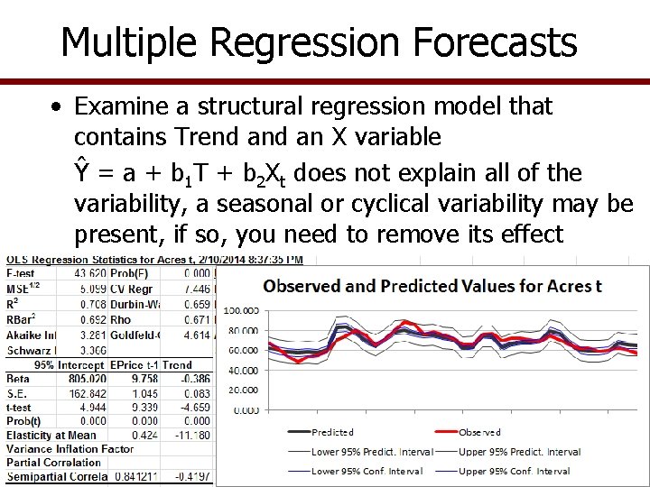
Multiple Regression Forecasts • Examine a structural regression model that contains Trend an X variable Ŷ = a + b 1 T + b 2 Xt does not explain all of the variability, a seasonal or cyclical variability may be present, if so, you need to remove its effect

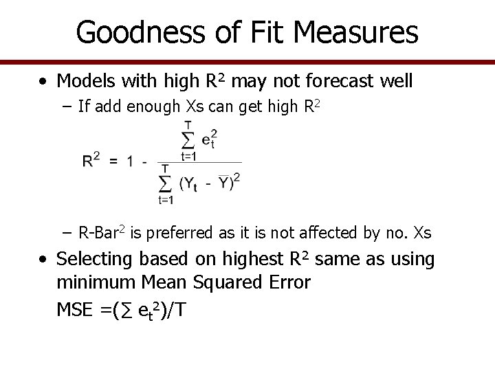
Goodness of Fit Measures • Models with high R 2 may not forecast well – If add enough Xs can get high R 2 – R-Bar 2 is preferred as it is not affected by no. Xs • Selecting based on highest R 2 same as using minimum Mean Squared Error MSE =(∑ et 2)/T

Goodness of Fit Measures • Models with high R 2 may not forecast well – If add enough Xs can get high R 2 – R-Bar 2 is preferred as it is not affected by no. Xs • Selecting based on highest R 2 same as using minimum Mean Squared Error MSE =(∑ et 2)/T

Goodness of Fit Measures • I like to follow these simple rules, in this order – Correct parameter signs based on sound economic theory for al variables • For supply beta on price must be positive, etc. – Student t ratios greater than 2. 0 and/or P values for betas less than 0. 05 – F ratio larger than 20. 0 – R 2 as large as you can get – MAPE (mean absolute percent error) less than 0. 1 (or 10%) • For large models OLS is preferred

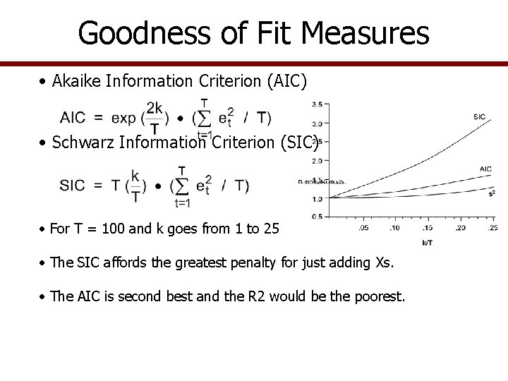
Goodness of Fit Measures • Akaike Information Criterion (AIC) • Schwarz Information Criterion (SIC) • For T = 100 and k goes from 1 to 25 • The SIC affords the greatest penalty for just adding Xs. • The AIC is second best and the R 2 would be the poorest.

Goodness of Fit Measures • Summary of goodness of fit measures – SIC, AIC, and S 2 are sensitive to both k and T – The S 2 is small and rises slowly as k/T increases – AIC and SIC rise faster as k/T increases – SIC is most sensitive to k/T increases

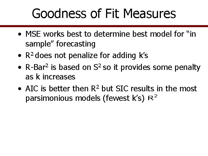
Goodness of Fit Measures • MSE works best to determine best model for “in sample” forecasting • R 2 does not penalize for adding k’s • R-Bar 2 is based on S 2 so it provides some penalty as k increases • AIC is better then R 2 but SIC results in the most parsimonious models (fewest k’s)