Multiple Regression Dummy Variables Multicollinearity Interaction Effects Heteroscedasticity

Lecture Objectives You should be able to : 1. Convert categorical variables into dummies. 2. Identify and eliminate Multicollinearity. 3. Use interaction terms and interpret their coefficients. 4. Identify heteroscedasticity.

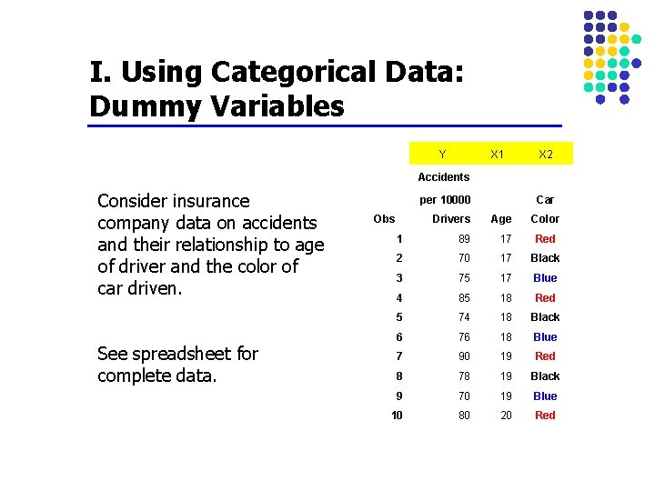
I. Using Categorical Data: Dummy Variables Y X 1 X 2 Accidents Consider insurance company data on accidents and their relationship to age of driver and the color of car driven. See spreadsheet for complete data. per 10000 Obs Car Drivers Age Color 1 89 17 Red 2 70 17 Black 3 75 17 Blue 4 85 18 Red 5 74 18 Black 6 76 18 Blue 7 90 19 Red 8 78 19 Black 9 70 19 Blue 10 80 20 Red

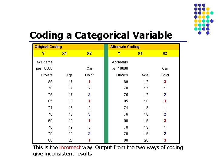
Coding a Categorical Variable Original Coding Y Alternate Coding X 1 X 2 Accidents Y X 1 X 2 Accidents per 10000 Car Drivers Age 89 17 70 Color per 10000 Car Drivers Age Color 1 89 17 3 17 2 70 17 1 75 17 3 75 17 2 85 18 1 85 18 3 74 18 2 74 18 1 76 18 3 76 18 2 90 19 1 90 19 3 78 19 2 78 19 1 70 19 3 70 19 2 80 20 1 80 20 3 This is the incorrect way. Output from the two ways of coding give inconsistent results.

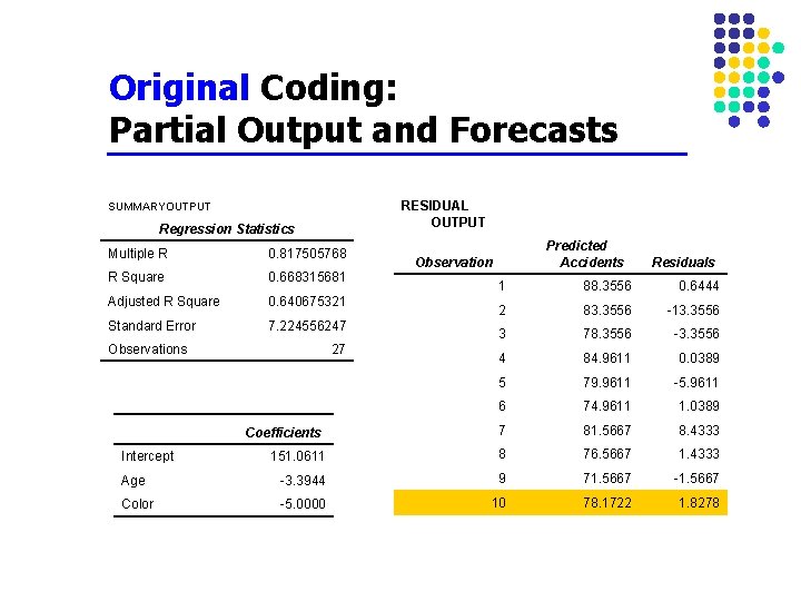
Original Coding: Partial Output and Forecasts RESIDUAL OUTPUT SUMMARYOUTPUT Regression Statistics Multiple R 0. 817505768 R Square 0. 668315681 Adjusted R Square 0. 640675321 Standard Error 7. 224556247 Predicted Accidents Observation Residuals 1 88. 3556 0. 6444 2 83. 3556 -13. 3556 3 78. 3556 -3. 3556 4 84. 9611 0. 0389 5 79. 9611 -5. 9611 6 74. 9611 1. 0389 7 81. 5667 8. 4333 151. 0611 8 76. 5667 1. 4333 Age -3. 3944 9 71. 5667 -1. 5667 Color -5. 0000 10 78. 1722 1. 8278 Observations 27 Coefficients Intercept

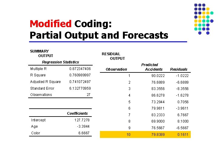
Modified Coding: Partial Output and Forecasts SUMMARY OUTPUT RESIDUAL OUTPUT Regression Statistics Predicted Accidents Multiple R 0. 872347406 R Square 0. 760989997 1 90. 0222 -1. 0222 Adjusted R Square 0. 741072497 2 76. 6889 -6. 6889 Standard Error 6. 132770959 3 83. 3556 -8. 3556 27 4 86. 6278 -1. 6278 5 73. 2944 0. 7056 6 79. 9611 -3. 9611 7 83. 2333 6. 7667 127. 7278 8 69. 9000 8. 1000 -3. 3944 9 76. 5667 -6. 5667 6. 6667 10 79. 8389 0. 1611 Observations Coefficients Intercept Age Color Observation Residuals

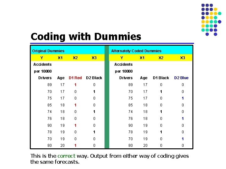
Coding with Dummies Original Dummies Y X 1 Alternately Coded Dummies X 2 X 3 Y X 1 Accidents per 10000 Drivers Age D 1 Red D 2 Black 89 17 1 70 17 75 X 2 X 3 D 1 Black D 2 Blue Drivers Age 0 89 17 0 0 0 1 70 17 1 0 17 0 0 75 17 0 1 85 18 1 0 85 18 0 0 74 18 0 1 74 18 1 0 76 18 0 1 90 19 1 0 90 19 0 0 78 19 0 1 78 19 1 0 70 19 0 1 80 20 1 0 80 20 0 0 This is the correct way. Output from either way of coding gives the same forecasts.

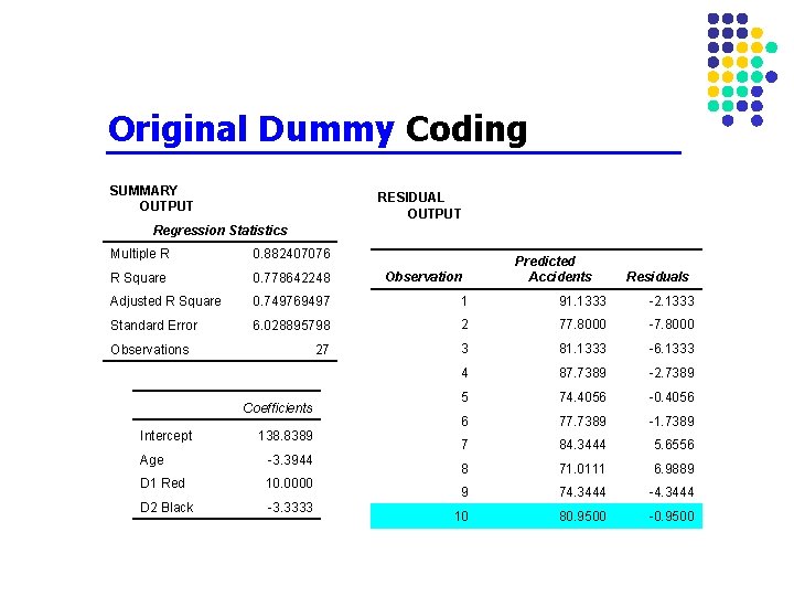
Original Dummy Coding SUMMARY OUTPUT RESIDUAL OUTPUT Regression Statistics Multiple R 0. 882407076 R Square 0. 778642248 Adjusted R Square 0. 749769497 1 91. 1333 -2. 1333 Standard Error 6. 028895798 2 77. 8000 -7. 8000 27 3 81. 1333 -6. 1333 4 87. 7389 -2. 7389 5 74. 4056 -0. 4056 6 77. 7389 -1. 7389 7 84. 3444 5. 6556 8 71. 0111 6. 9889 9 74. 3444 -4. 3444 10 80. 9500 -0. 9500 Observations Coefficients Intercept 138. 8389 Age -3. 3944 D 1 Red 10. 0000 D 2 Black -3. 3333 Observation Predicted Accidents Residuals

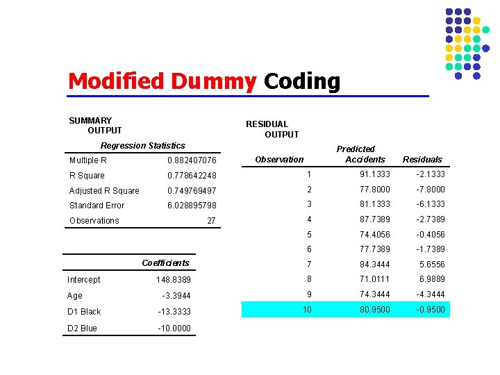
Modified Dummy Coding SUMMARY OUTPUT RESIDUAL OUTPUT Regression Statistics Predicted Accidents Observation Residuals Multiple R 0. 882407076 R Square 0. 778642248 1 91. 1333 -2. 1333 Adjusted R Square 0. 749769497 2 77. 8000 -7. 8000 Standard Error 6. 028895798 3 81. 1333 -6. 1333 27 4 87. 7389 -2. 7389 5 74. 4056 -0. 4056 6 77. 7389 -1. 7389 Coefficients 7 84. 3444 5. 6556 148. 8389 8 71. 0111 6. 9889 -3. 3944 9 74. 3444 -4. 3444 D 1 Black -13. 3333 10 80. 9500 -0. 9500 D 2 Blue -10. 0000 Observations Intercept Age

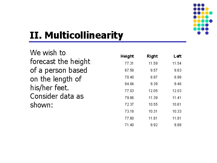
II. Multicollinearity We wish to forecast the height of a person based on the length of his/her feet. Consider data as shown: Height Right Left 77. 31 11. 59 11. 54 67. 58 9. 57 9. 63 70. 40 8. 97 8. 98 64. 84 9. 39 9. 46 77. 03 12. 05 12. 03 79. 66 11. 39 11. 41 72. 37 10. 55 10. 61 73. 18 10. 31 10. 33 77. 60 11. 81 71. 40 9. 92 9. 88

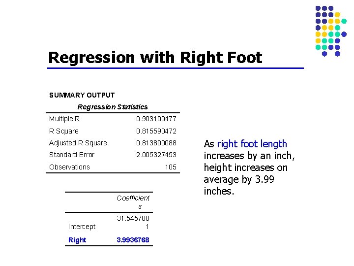
Regression with Right Foot SUMMARY OUTPUT Regression Statistics Multiple R 0. 903100477 R Square 0. 815590472 Adjusted R Square 0. 813800088 Standard Error 2. 005327453 Observations 105 Coefficient s Intercept 31. 545700 1 Right 3. 9936768 As right foot length increases by an inch, height increases on average by 3. 99 inches.

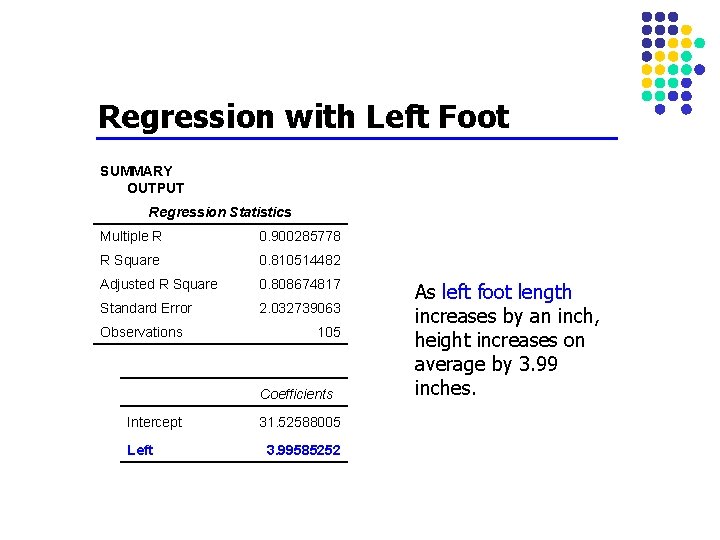
Regression with Left Foot SUMMARY OUTPUT Regression Statistics Multiple R 0. 900285778 R Square 0. 810514482 Adjusted R Square 0. 808674817 Standard Error 2. 032739063 Observations 105 Coefficients Intercept Left 31. 52588005 3. 99585252 As left foot length increases by an inch, height increases on average by 3. 99 inches.

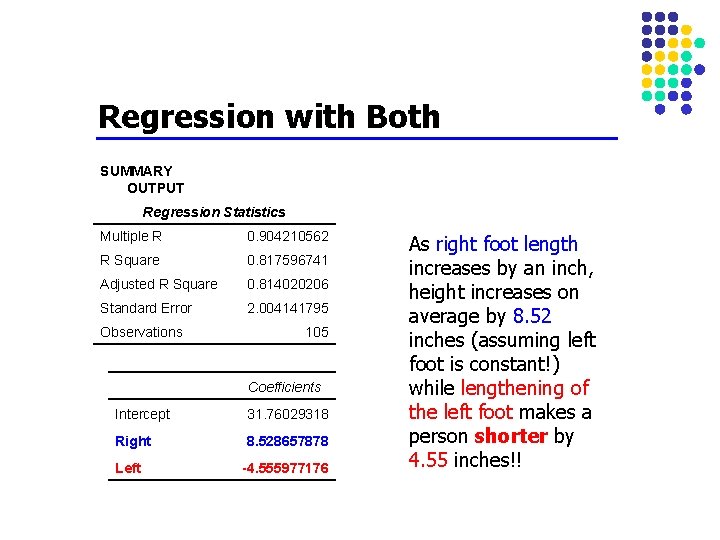
Regression with Both SUMMARY OUTPUT Regression Statistics Multiple R 0. 904210562 R Square 0. 817596741 Adjusted R Square 0. 814020206 Standard Error 2. 004141795 Observations 105 Coefficients Intercept 31. 76029318 Right 8. 528657878 Left -4. 555977176 As right foot length increases by an inch, height increases on average by 8. 52 inches (assuming left foot is constant!) while lengthening of the left foot makes a person shorter by 4. 55 inches!!

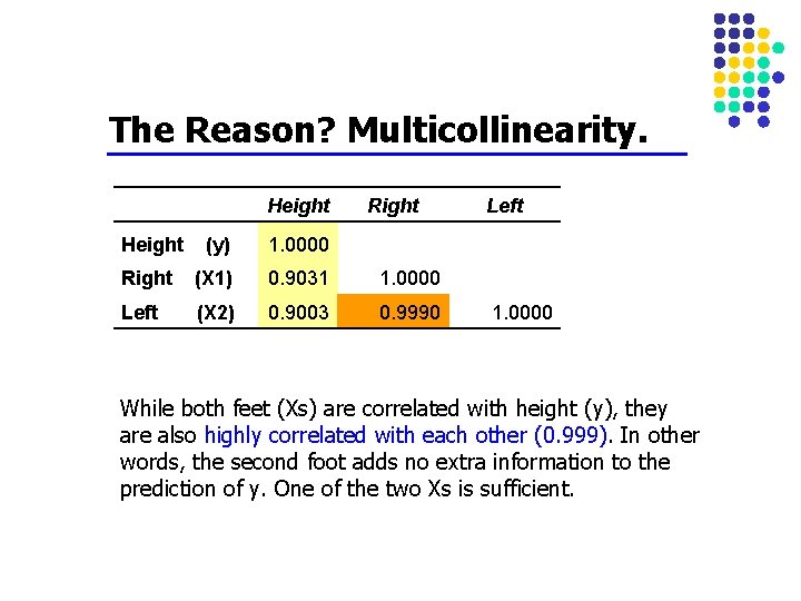
The Reason? Multicollinearity. Height Right Height (y) 1. 0000 Right (X 1) 0. 9031 1. 0000 Left (X 2) 0. 9003 0. 9990 Left 1. 0000 While both feet (Xs) are correlated with height (y), they are also highly correlated with each other (0. 999). In other words, the second foot adds no extra information to the prediction of y. One of the two Xs is sufficient.

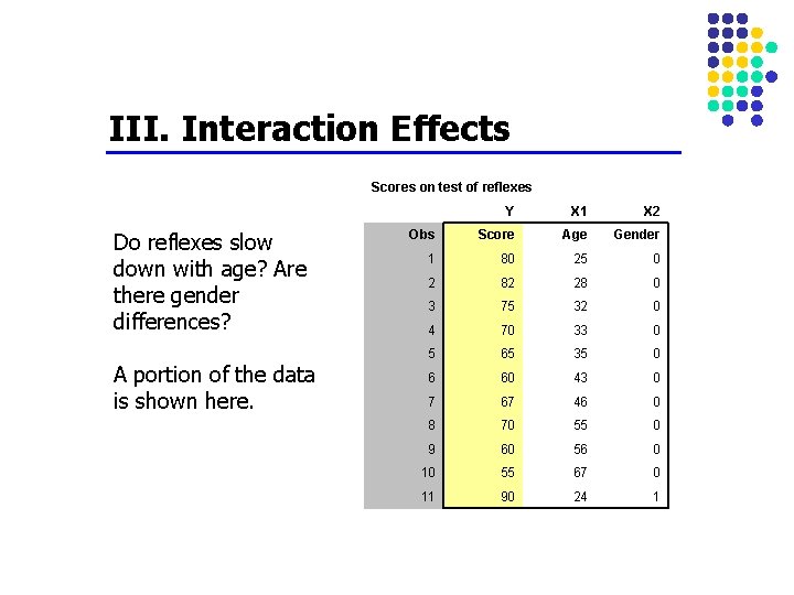
III. Interaction Effects Scores on test of reflexes Do reflexes slow down with age? Are there gender differences? A portion of the data is shown here. Y X 1 X 2 Obs Score Age Gender 1 80 25 0 2 82 28 0 3 75 32 0 4 70 33 0 5 65 35 0 6 60 43 0 7 67 46 0 8 70 55 0 9 60 56 0 10 55 67 0 11 90 24 1

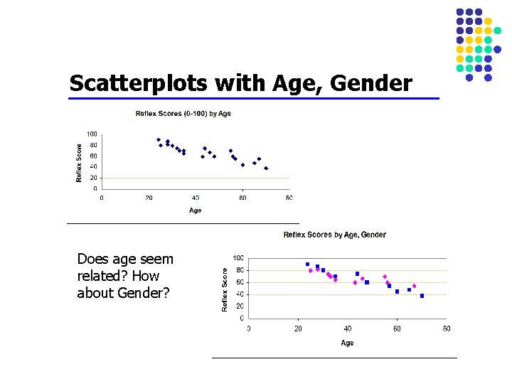
Scatterplots with Age, Gender Does age seem related? How about Gender?

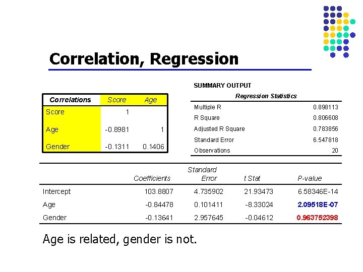
Correlation, Regression SUMMARY OUTPUT Correlations Score Regression Statistics Age 1 Age -0. 8981 1 Gender -0. 1311 0. 1406 Coefficients Multiple R 0. 898113 R Square 0. 806608 Adjusted R Square 0. 783856 Standard Error 6. 547818 Observations Standard Error 20 t Stat P-value Intercept 103. 8807 4. 735902 21. 93473 6. 58346 E-14 Age -0. 84478 0. 101411 -8. 33024 2. 09518 E-07 Gender -0. 13641 2. 957645 -0. 04612 0. 963752398 Age is related, gender is not.

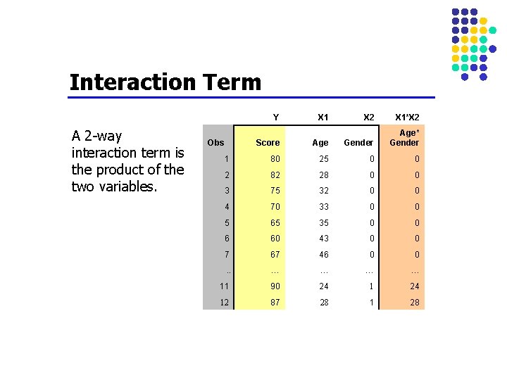
Interaction Term A 2 -way interaction term is the product of the two variables. Y X 1 X 2 X 1*X 2 Score Age Gender Age* Gender 1 80 25 0 0 2 82 28 0 0 3 75 32 0 0 4 70 33 0 0 5 65 35 0 0 6 60 43 0 0 7 67 46 0 0 . . … … 11 90 24 12 87 28 1 28 Obs

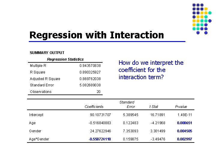
Regression with Interaction SUMMARY OUTPUT Regression Statistics Multiple R 0. 943570838 R Square 0. 890325927 Adjusted R Square 0. 869762038 Standard Error 5. 082689038 Observations 20 Coefficients Intercept Age Gender Age*Gender How do we interpret the coefficient for the interaction term? Standard Error t Stat P-value 90. 10731707 5. 389545 16. 71891 1. 49 E-11 -0. 516840883 0. 122483 -4. 21968 0. 000651 24. 27622946 7. 353093 3. 301499 0. 004505 -0. 558724118 0. 159875 -3. 49476 0. 002997

Meaning of Interaction X 1 and X 2 are said to interact with each other if the impact of X 1 on y changes as the value of X 2 changes. In this example, the impact of age (X 1) on reflexes (y) is different for males and females (changing values of X 2). Hence age and gender are said to interact. Explain how this is different from multicollinearity.

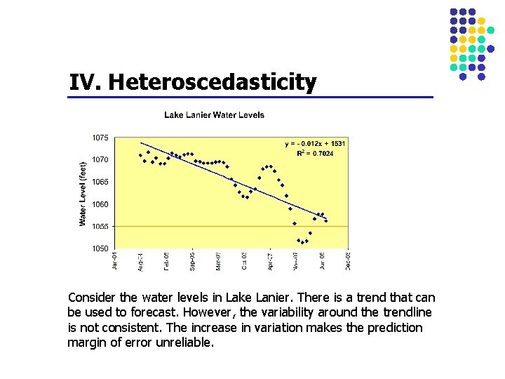
IV. Heteroscedasticity Consider the water levels in Lake Lanier. There is a trend that can be used to forecast. However, the variability around the trendline is not consistent. The increase in variation makes the prediction margin of error unreliable.

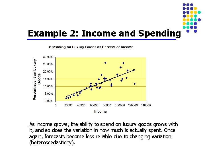
Example 2: Income and Spending As income grows, the ability to spend on luxury goods grows with it, and so does the variation in how much is actually spent. Once again, forecasts become less reliable due to changing variation (heteroscedasticity).

Solution When heteroscedasticity is identified, data may need to be transformed (change to a log scale, for instance) to reduce its impact. The type of transformation needed depends on the data.