Multiple Regression Analysis Estimation Multiple Regression Model y

Multiple Regression Analysis: Estimation

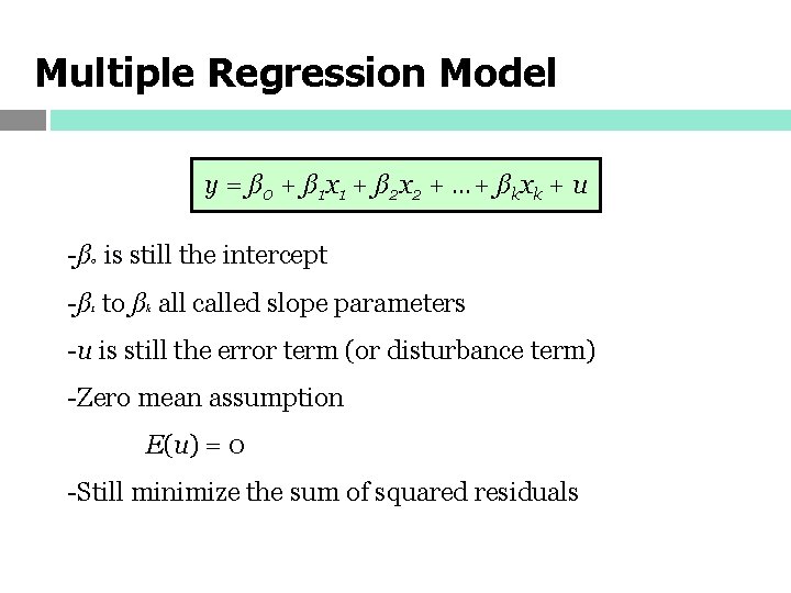
Multiple Regression Model y = ß 0 + ß 1 x 1 + ß 2 x 2 + …+ ßkxk + u -ß is still the intercept 0 -ß to ß all called slope parameters 1 k -u is still the error term (or disturbance term) -Zero mean assumption E(u) = 0 -Still minimize the sum of squared residuals

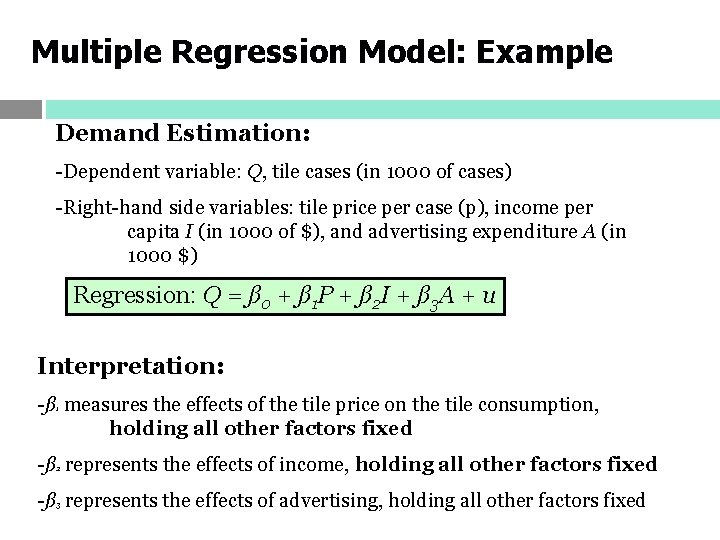
Multiple Regression Model: Example Demand Estimation: -Dependent variable: Q, tile cases (in 1000 of cases) -Right-hand side variables: tile price per case (p), income per capita I (in 1000 of $), and advertising expenditure A (in 1000 $) Regression: Q = ß 0 + ß 1 P + ß 2 I + ß 3 A + u Interpretation: -ß measures the effects of the tile price on the tile consumption, holding all other factors fixed 1 -ß represents the effects of income, holding all other factors fixed 2 -ß represents the effects of advertising, holding all other factors fixed 3

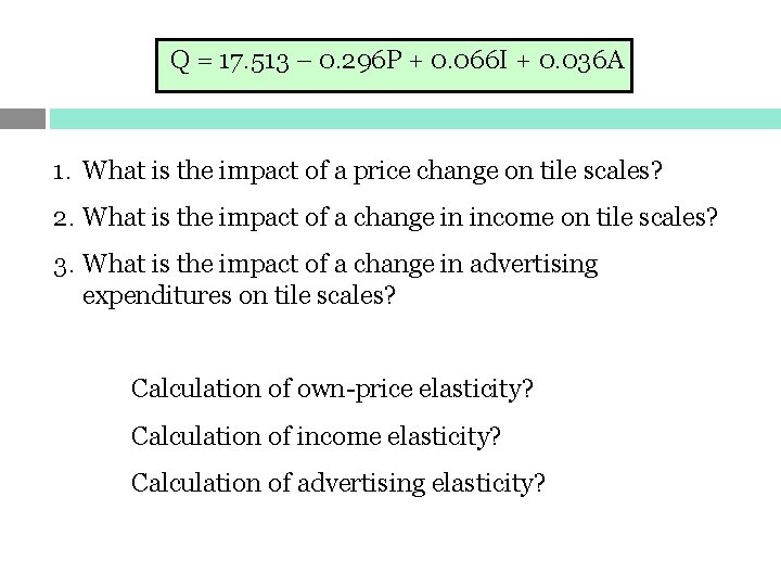
Q = 17. 513 – 0. 296 P + 0. 066 I + 0. 036 A 1. What is the impact of a price change on tile scales? 2. What is the impact of a change in income on tile scales? 3. What is the impact of a change in advertising expenditures on tile scales? Calculation of own-price elasticity? Calculation of income elasticity? Calculation of advertising elasticity?

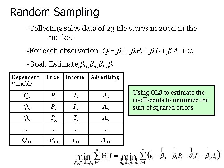
Random Sampling -Collecting sales data of 23 tile stores in 2002 in the market -For each observation, Q = ß + ß P + ß I + ß A + u i -Goal: Estimate ß , ß , ß 0 1 2 0 1 i 2 i 3 i i 3 Dependent Variable Price Income Advertising Q 1 P 1 I 1 A 1 Q 2 P 2 I 2 A 2 Q 3 P 3 I 3 A 3 … … Q 23 P 23 I 23 A 23 Using OLS to estimate the coefficients to minimize the sum of squared errors.

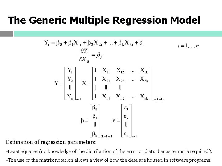
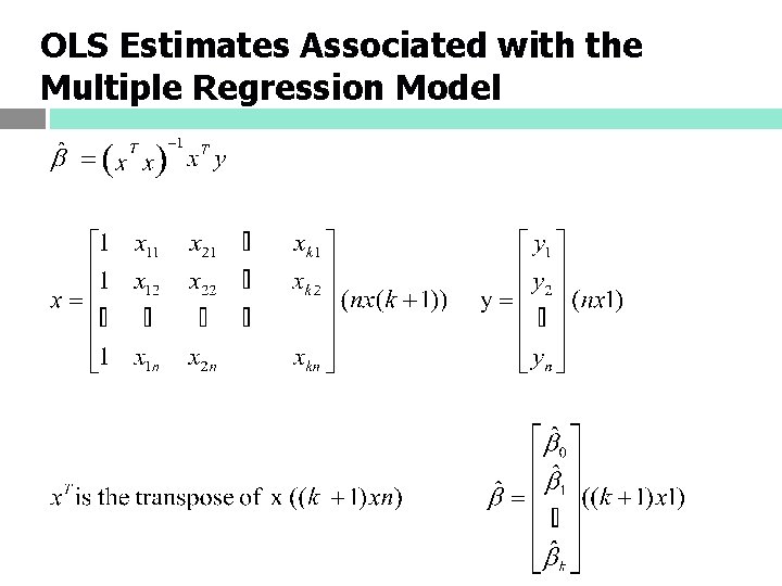
The Generic Multiple Regression Model Estimation of regression parameters: -Least Squares (no knowledge of the distribution of the error or disturbance terms is required). -The use of the matrix notation allows a view of how the data are housed in software programs.

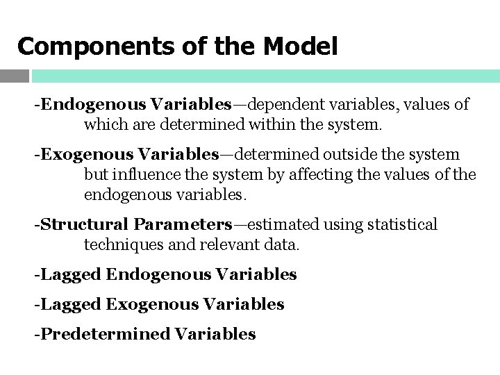
Components of the Model -Endogenous Variables—dependent variables, values of which are determined within the system. -Exogenous Variables—determined outside the system but influence the system by affecting the values of the endogenous variables. -Structural Parameters—estimated using statistical techniques and relevant data. -Lagged Endogenous Variables -Lagged Exogenous Variables -Predetermined Variables

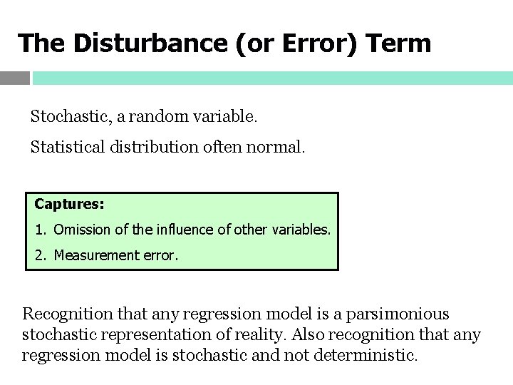
The Disturbance (or Error) Term Stochastic, a random variable. Statistical distribution often normal. Captures: 1. Omission of the influence of other variables. 2. Measurement error. Recognition that any regression model is a parsimonious stochastic representation of reality. Also recognition that any regression model is stochastic and not deterministic.

OLS Estimates Associated with the Multiple Regression Model

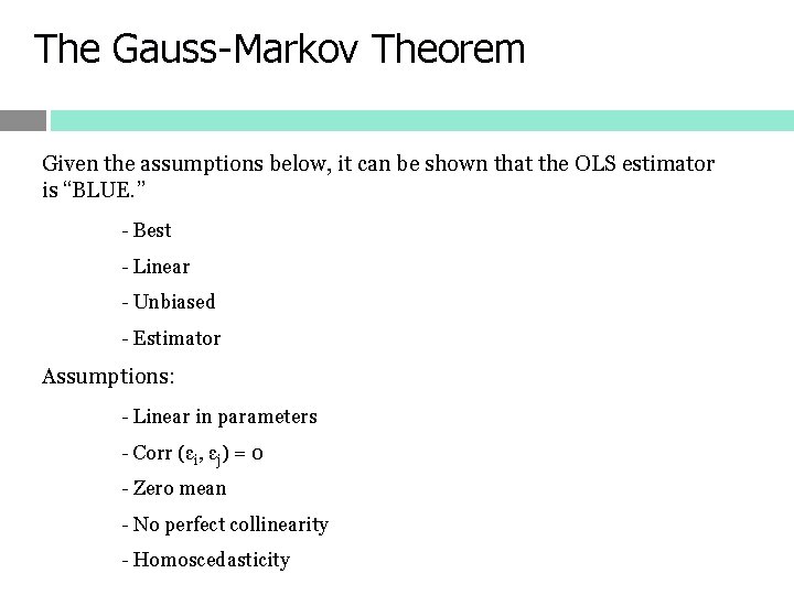
The Gauss-Markov Theorem Given the assumptions below, it can be shown that the OLS estimator is “BLUE. ” - Best - Linear - Unbiased - Estimator Assumptions: - Linear in parameters - Corr (εi, εj) = 0 - Zero mean - No perfect collinearity - Homoscedasticity

Communication and Aims for the Analyst

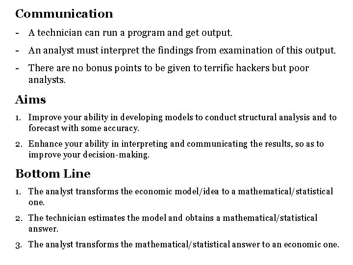
Communication - A technician can run a program and get output. - An analyst must interpret the findings from examination of this output. - There are no bonus points to be given to terrific hackers but poor analysts. Aims 1. Improve your ability in developing models to conduct structural analysis and to forecast with some accuracy. 2. Enhance your ability in interpreting and communicating the results, so as to improve your decision-making. Bottom Line 1. The analyst transforms the economic model/idea to a mathematical/statistical one. 2. The technician estimates the model and obtains a mathematical/statistical answer. 3. The analyst transforms the mathematical/statistical answer to an economic one.

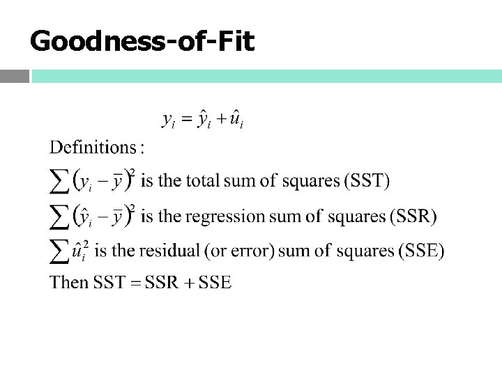
Goodness-of-Fit

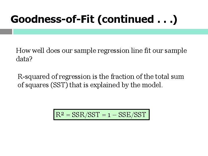
Goodness-of-Fit (continued. . . ) How well does our sample regression line fit our sample data? R-squared of regression is the fraction of the total sum of squares (SST) that is explained by the model. R² = SSR/SST = 1 – SSE/SST

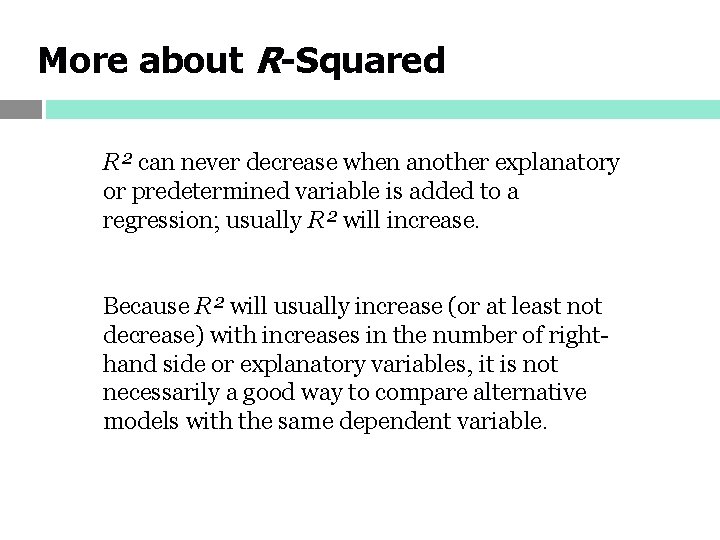
More about R-Squared R² can never decrease when another explanatory or predetermined variable is added to a regression; usually R² will increase. Because R² will usually increase (or at least not decrease) with increases in the number of righthand side or explanatory variables, it is not necessarily a good way to compare alternative models with the same dependent variable.

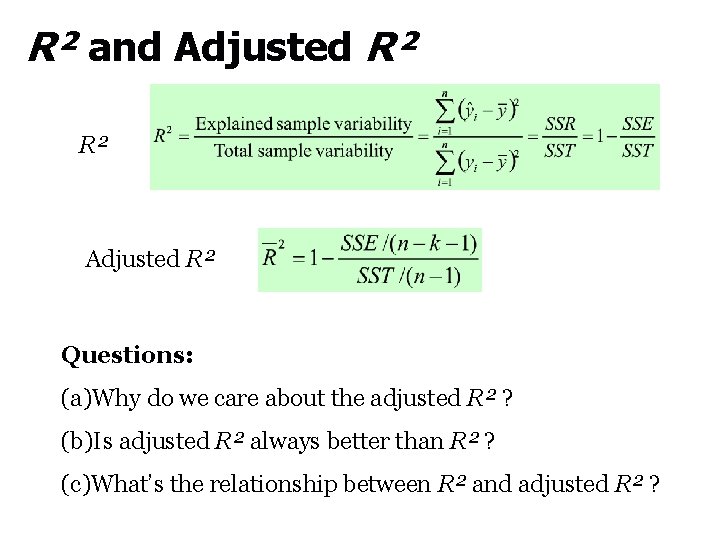
R² and Adjusted R² R² Adjusted R² Questions: (a)Why do we care about the adjusted R² ? (b)Is adjusted R² always better than R² ? (c)What’s the relationship between R² and adjusted R² ?

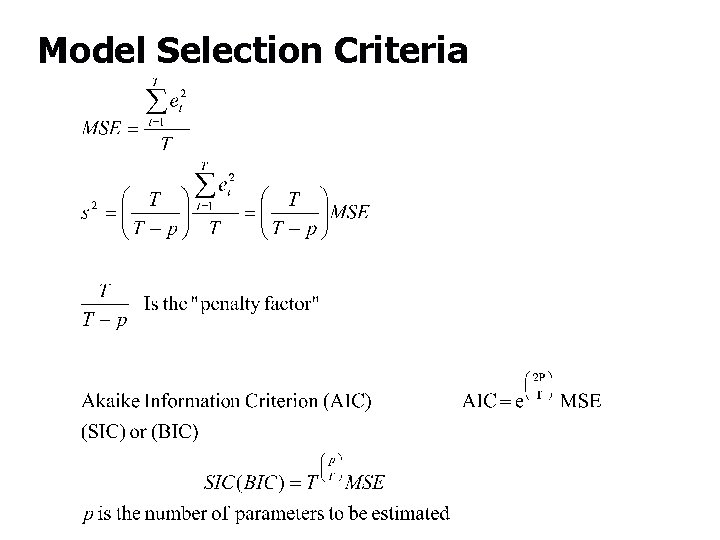
Model Selection Criteria

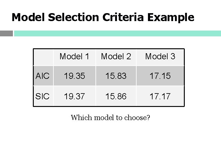
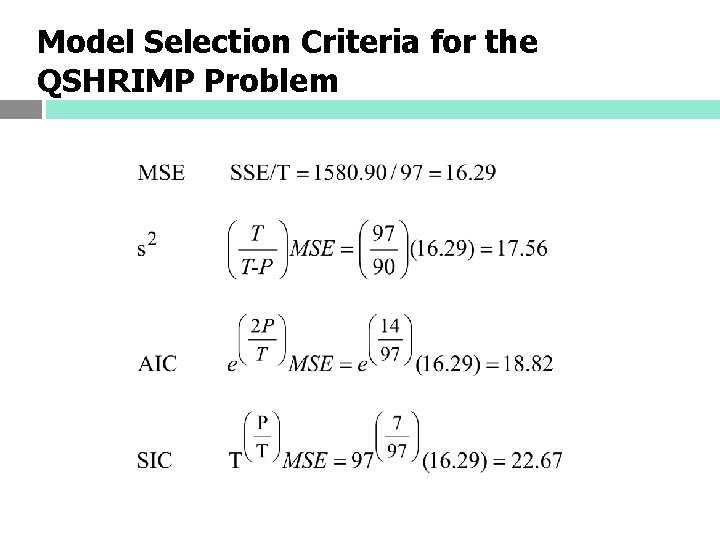
Model Selection Criteria Example Model 1 Model 2 Model 3 AIC 19. 35 15. 83 17. 15 SIC 19. 37 15. 86 17. 17 Which model to choose?

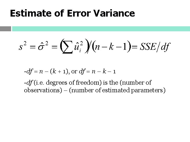
Estimate of Error Variance -df = n – (k + 1), or df = n – k – 1 -df (i. e. degrees of freedom) is the (number of observations) – (number of estimated parameters)

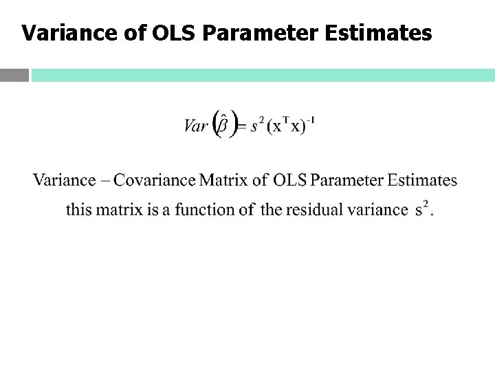
Variance of OLS Parameter Estimates

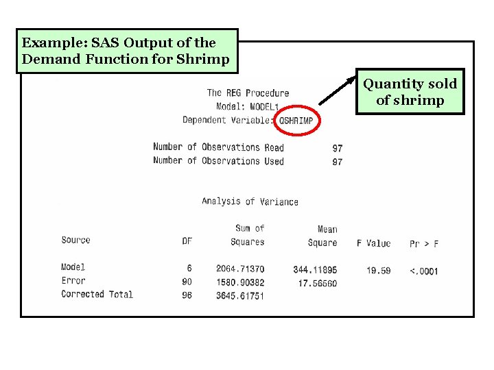
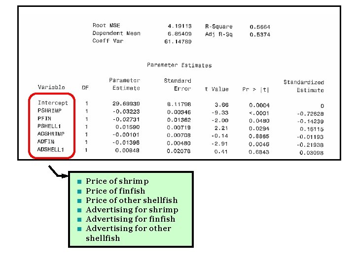
Example: SAS Output of the Demand Function for Shrimp Quantity sold of shrimp

■ ■ ■ Price of shrimp Price of finfish Price of other shellfish Advertising for shrimp Advertising for finfish Advertising for other shellfish

Model Selection Criteria for the QSHRIMP Problem