Multiple Regression 1 Sociology 5811 Lecture 22 Copyright

Multiple Regression 1 Sociology 5811 Lecture 22 Copyright © 2005 by Evan Schofer Do not copy or distribute without permission

Announcements • None!

Multiple Regression • Question: What if a dependent variable is affected by more than one independent variable? • Strategy #1: Do separate bivariate regressions – One regression for each independent variable • This yields separate slope estimates for each independent variable – Bivariate slope estimates implicitly assume that neither independent variable mediates the other – In reality, there might be no effect of family wealth over and above education

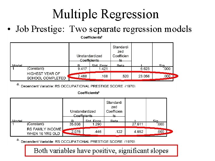
Multiple Regression • Job Prestige: Two separate regression models Both variables have positive, significant slopes

Multiple Regression • Idea #2: Use Multiple Regression • Multiple regression can examine “partial” relationships – Partial = Relationships after the effects of other variables have been “controlled” (taken into account) • This lets you determine the effects of variables “over and above” other variables – And shows the relative impact of different factors on a dependent variable • And, you can use several independent variables to improve your predictions of the dependent var

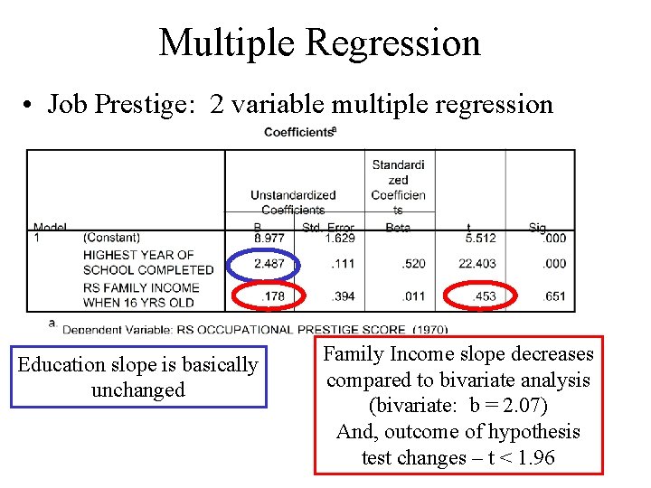
Multiple Regression • Job Prestige: 2 variable multiple regression Education slope is basically unchanged Family Income slope decreases compared to bivariate analysis (bivariate: b = 2. 07) And, outcome of hypothesis test changes – t < 1. 96

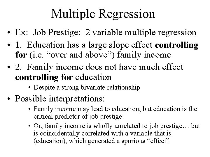
Multiple Regression • Ex: Job Prestige: 2 variable multiple regression • 1. Education has a large slope effect controlling for (i. e. “over and above”) family income • 2. Family income does not have much effect controlling for education • Despite a strong bivariate relationship • Possible interpretations: • Family income may lead to education, but education is the critical predictor of job prestige • Or, family income is wholly unrelated to job prestige… but is coincidentally correlated with a variable that is (education), which generated a spurious “effect”.

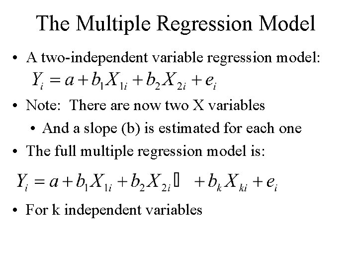
The Multiple Regression Model • A two-independent variable regression model: • Note: There are now two X variables • And a slope (b) is estimated for each one • The full multiple regression model is: • For k independent variables

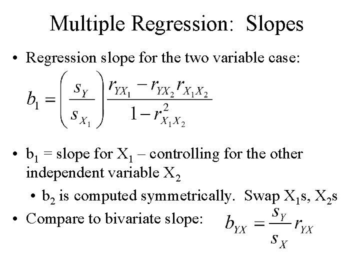
Multiple Regression: Slopes • Regression slope for the two variable case: • b 1 = slope for X 1 – controlling for the other independent variable X 2 • b 2 is computed symmetrically. Swap X 1 s, X 2 s • Compare to bivariate slope:

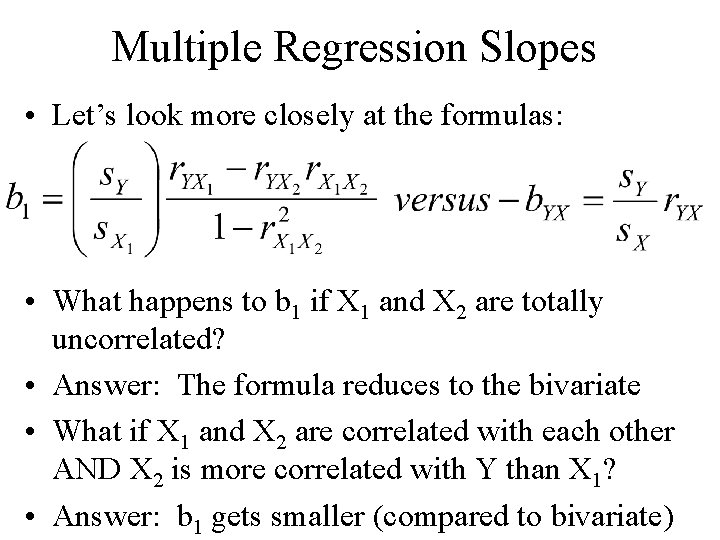
Multiple Regression Slopes • Let’s look more closely at the formulas: • What happens to b 1 if X 1 and X 2 are totally uncorrelated? • Answer: The formula reduces to the bivariate • What if X 1 and X 2 are correlated with each other AND X 2 is more correlated with Y than X 1? • Answer: b 1 gets smaller (compared to bivariate)

Regression Slopes • So, if two variables (X 1, X 2) are correlated and both predict Y: • The X variable that is more correlated with Y will have a higher slope in multivariate regression – The slope of the less-correlated variable will shrink • Thus, slopes for each variable are adjusted to how well the other variable predicts Y – It is the slope “controlling” for other variables

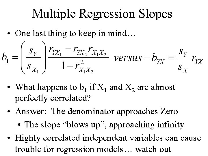
Multiple Regression Slopes • One last thing to keep in mind… • What happens to b 1 if X 1 and X 2 are almost perfectly correlated? • Answer: The denominator approaches Zero • The slope “blows up”, approaching infinity • Highly correlated independent variables can cause trouble for regression models… watch out

Interpreting Results • (Over)Simplified rules for interpretation – Assumes good sample, measures, models, etc. • Multivariate regression with two variables: A, B • If slopes of A, B are the same as bivariate, then each has an independent effect • If A remains large, B shrinks to zero we typically conclude that effect of B was spurious, or operates through A • If both A and B shrink a little, each has an effect, but some overlap or mediation is occurring

Interpreting Multivariate Results • Things to watch out for: • 1. Remember: Correlation is not causation – Ability to “control” for many variables can help detect spurious relationships… but it isn’t perfect. – Be aware that other (omitted) variables may be affecting your model. Don’t over-interpret results. • 2. Reverse causality – Many sociological processes involve bi-directional causality. Regression slopes (and correlations) do not identify which variable “causes” the other. • Ex: self-esteem and test scores.

Standardized Regression Coefficients • Regression slopes reflect the units of the independent variables • Question: How do you compare how “strong” the effects of two variables if they have totally different units? • Example: Education, family wealth, job prestige – Education measured in years, b = 2. 5 – Family wealth measured on 1 -5 scale, b =. 18 – Which is a “bigger” effect? Units aren’t comparable! • Answer: Create “standardized” coefficients

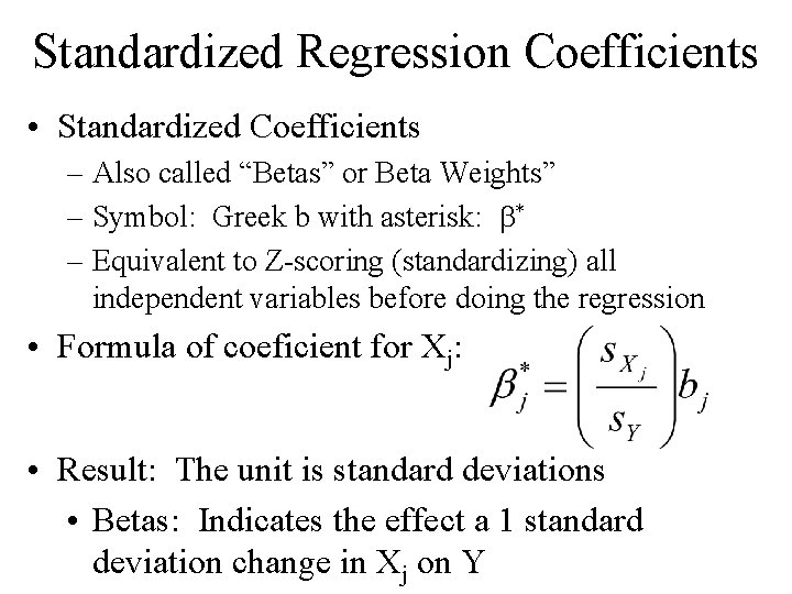
Standardized Regression Coefficients • Standardized Coefficients – Also called “Betas” or Beta Weights” – Symbol: Greek b with asterisk: b* – Equivalent to Z-scoring (standardizing) all independent variables before doing the regression • Formula of coeficient for Xj: • Result: The unit is standard deviations • Betas: Indicates the effect a 1 standard deviation change in Xj on Y

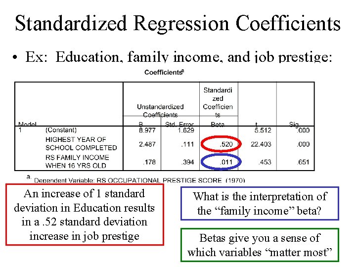
Standardized Regression Coefficients • Ex: Education, family income, and job prestige: An increase of 1 standard deviation in Education results in a. 52 standard deviation increase in job prestige What is the interpretation of the “family income” beta? Betas give you a sense of which variables “matter most”

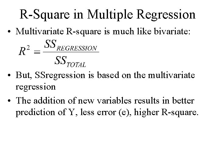
R-Square in Multiple Regression • Multivariate R-square is much like bivariate: • But, SSregression is based on the multivariate regression • The addition of new variables results in better prediction of Y, less error (e), higher R-square.

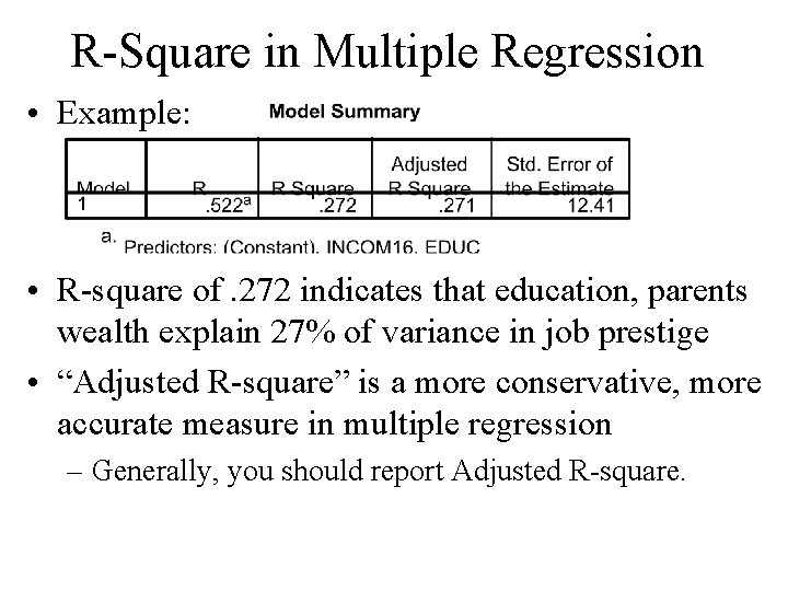
R-Square in Multiple Regression • Example: • R-square of. 272 indicates that education, parents wealth explain 27% of variance in job prestige • “Adjusted R-square” is a more conservative, more accurate measure in multiple regression – Generally, you should report Adjusted R-square.

Dummy Variables • Question: How can we incorporate nominal variables (e. g. , race, gender) into regression? • Option 1: Analyze each sub-group separately – Generates different slope, constant for each group • Option 2: Dummy variables – “Dummy” = a dichotomous variables coded to indicate the presence or absence of something – Absence coded as zero, presence coded as 1.

Dummy Variables • Strategy: Create a separate dummy variable for all nominal categories • Ex: Gender – make female & male variables – DFEMALE: coded as 1 for all women, zero for men – DMALE: coded as 1 for all men • Next: Include all but one dummy variables into a multiple regression model • If two dummies, include 1; If 5 dummies, include 4.

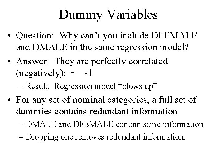
Dummy Variables • Question: Why can’t you include DFEMALE and DMALE in the same regression model? • Answer: They are perfectly correlated (negatively): r = -1 – Result: Regression model “blows up” • For any set of nominal categories, a full set of dummies contains redundant information – DMALE and DFEMALE contain same information – Dropping one removes redundant information.

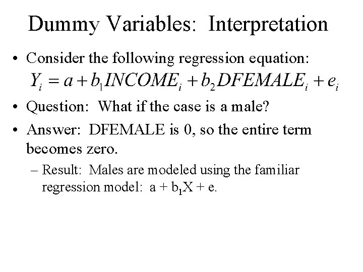
Dummy Variables: Interpretation • Consider the following regression equation: • Question: What if the case is a male? • Answer: DFEMALE is 0, so the entire term becomes zero. – Result: Males are modeled using the familiar regression model: a + b 1 X + e.

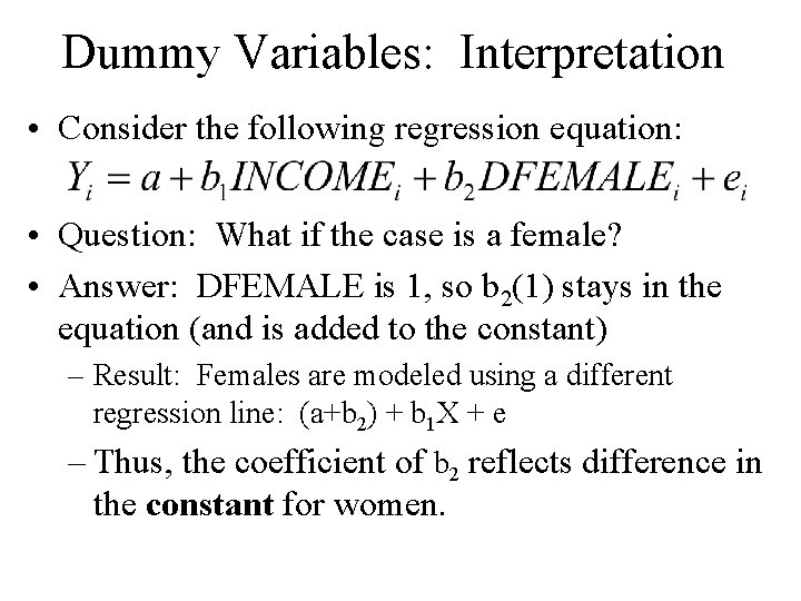
Dummy Variables: Interpretation • Consider the following regression equation: • Question: What if the case is a female? • Answer: DFEMALE is 1, so b 2(1) stays in the equation (and is added to the constant) – Result: Females are modeled using a different regression line: (a+b 2) + b 1 X + e – Thus, the coefficient of b 2 reflects difference in the constant for women.

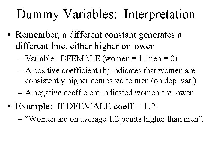
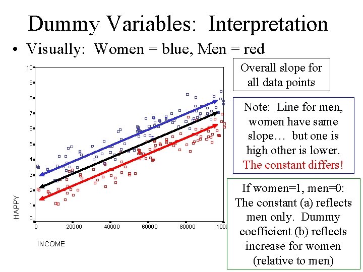
Dummy Variables: Interpretation • Remember, a different constant generates a different line, either higher or lower – Variable: DFEMALE (women = 1, men = 0) – A positive coefficient (b) indicates that women are consistently higher compared to men (on dep. var. ) – A negative coefficient indicated women are lower • Example: If DFEMALE coeff = 1. 2: – “Women are on average 1. 2 points higher than men”.

Dummy Variables: Interpretation • Visually: Women = blue, Men = red Overall slope for all data points 10 9 8 Note: Line for men, women have same slope… but one is high other is lower. The constant differs! 7 6 5 4 3 HAPPY 2 1 0 0 INCOME 20000 40000 60000 80000 If women=1, men=0: The constant (a) reflects men only. Dummy 100000 coefficient (b) reflects increase for women (relative to men)

Dummy Variables • What if you want to compare more than 2 groups? • Example: Race – Coded 1=white, 2=black, 3=other (like GSS) • Make 3 dummy variables: – “DWHITE” is 1 for whites, 0 for everyone else – “DBLACK” is 1 for Af. Am. , 0 for everyone else – “DOTHER” is 1 for “others”, 0 for everyone else • Then, include two of the three variables in the multiple regression model.

Dummy Variables: Interpretation • Ex: Job Prestige • Negative coefficient for DBLACK indicates a lower level of job prestige compared to whites – T- and P-values indicate if difference is significant.

Dummy Variables: Interpretation • Comments: • 1. Dummy coefficients shouldn’t be called slopes – Referring to the “slope” of gender doesn’t make sense – Rather, it is the difference in the constant (or “level”) • 2. The contrast is always with the nominal category that was left out of the equation – If DFEMALE is included, the contrast is with males – If DBLACK, DOTHER are included, coefficients reflect difference in constant compared to whites.

Interaction Terms • Question: What if you suspect that a variable has a totally different slope for two different subgroups in your data? • Example: Income and Happiness – Perhaps men are more materialistic -- an extra dollar increases their happiness a lot – If women are less materialistic, each dollar has a smaller effect on income (compared to men) • Issue isn’t men = “more” or “less” than women – Rather, the slope of a variable (income) differs across groups

Interaction Terms • Issue isn’t men = “more” or “less” than women – Rather, the slope of a variable coefficient (for income) differs across groups • Again, we want to specify a different regression line for each group – We want lines with different slopes, not parallel lines that are higher or lower.

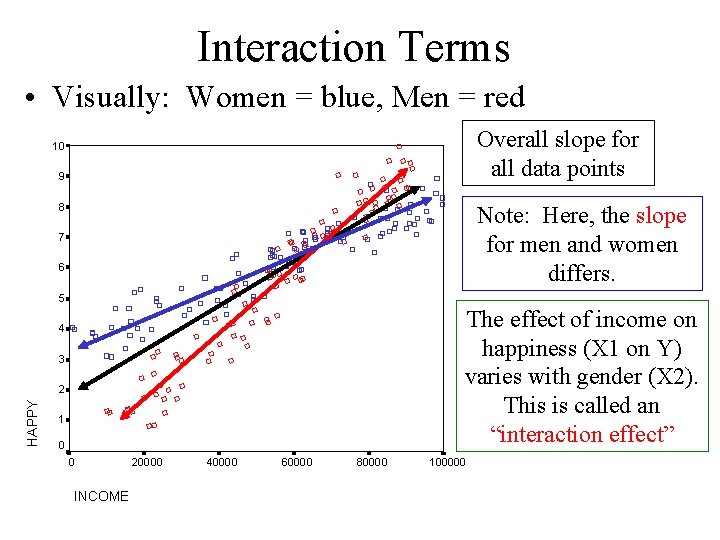
Interaction Terms • Visually: Women = blue, Men = red Overall slope for all data points 10 9 8 Note: Here, the slope for men and women differs. 7 6 5 The effect of income on happiness (X 1 on Y) varies with gender (X 2). This is called an “interaction effect” 4 3 HAPPY 2 1 0 0 INCOME 20000 40000 60000 80000 100000

Interaction Terms • Interaction effects: Differences in the relationship (slope) between two variables for each category of a third variable • Option #1: Analyze each group separately • Option #2: Multiply the two variables of interest: (DFEMALE, INCOME) to create a new variable – Called: DFEMALE*INCOME – Add that variable to the multiple regression model.

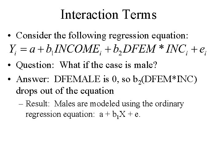
Interaction Terms • Consider the following regression equation: • Question: What if the case is male? • Answer: DFEMALE is 0, so b 2(DFEM*INC) drops out of the equation – Result: Males are modeled using the ordinary regression equation: a + b 1 X + e.

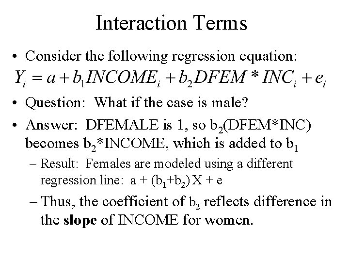
Interaction Terms • Consider the following regression equation: • Question: What if the case is male? • Answer: DFEMALE is 1, so b 2(DFEM*INC) becomes b 2*INCOME, which is added to b 1 – Result: Females are modeled using a different regression line: a + (b 1+b 2) X + e – Thus, the coefficient of b 2 reflects difference in the slope of INCOME for women.

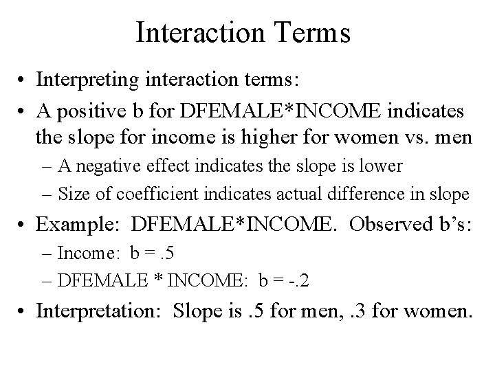
Interaction Terms • Interpreting interaction terms: • A positive b for DFEMALE*INCOME indicates the slope for income is higher for women vs. men – A negative effect indicates the slope is lower – Size of coefficient indicates actual difference in slope • Example: DFEMALE*INCOME. Observed b’s: – Income: b =. 5 – DFEMALE * INCOME: b = -. 2 • Interpretation: Slope is. 5 for men, . 3 for women.

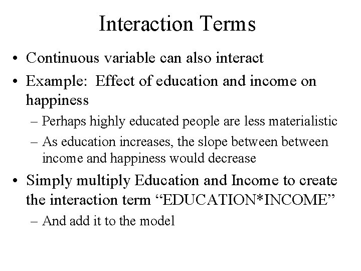
Interaction Terms • Continuous variable can also interact • Example: Effect of education and income on happiness – Perhaps highly educated people are less materialistic – As education increases, the slope between income and happiness would decrease • Simply multiply Education and Income to create the interaction term “EDUCATION*INCOME” – And add it to the model

Interaction Terms • How do you interpret continuous variable interactions? • Example: EDUCATION*INCOME: Coefficient = 2. 0 • Answer: For each unit change in education, the slope of income vs. happiness increases by 2 – Note: coefficient is symmetrical: For each unit change in income, education slope increases by 2 – Dummy interactions result in slopes for each group – Continuous interactions result in many slopes • Each category of education*income has a different slope.

Interaction Terms • Comments: • 1. If you make an interaction you should also include the component variables in the model: – A model with “DFEMALE * INCOME” should also include DFEMALE and INCOME – There is some debate on this issue… but that is the safest course of action • 2. Sometimes interaction terms are highly correlated with its components • Watch out for that.

Interaction Terms • Question: Can you think of examples of two variables that might interact? • Either from your final project? Or anything else?