Multiple Linear Regression Matrix Formulation Let x x

Multiple Linear Regression Matrix Formulation Let x = (x 1, x 2, … , xn)′ be a n 1 column vector and let g(x) be a scalar function of x. Then, by definition,

For example, let Let a = (a 1, a 2, … , a n)′ be a n 1 column vector of constants. It is easy to verify that and that, for symmetrical A (n n)

Theory of Multiple Regression Suppose we have response variables Yi , i = 1, 2, … , n and k explanatory variables/predictors X 1, X 2, … , X k. i = 1, 2, … , n There are k+2 parameters b 0 , b 1 , b 2 , …, bk and σ2

X is called the design matrix

OLS (ordinary least squares) estimation

Fitted values are given by H is called the “hat matrix” (… it puts the hats on the Y’s)

The error sum of squares, SSRES , is The estimate of s 2 is based on this.

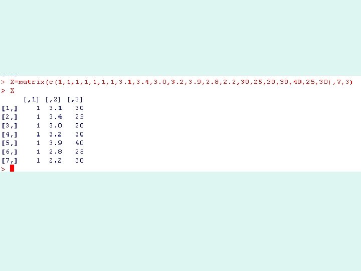
Example: Find a model of the form for the data below. y x 1 x 2 3. 5 3. 1 30 3. 2 3. 4 25 3. 0 20 2. 9 3. 2 30 4. 0 3. 9 40 2. 5 2. 8 25 2. 3 2. 2 30

X is called the design matrix

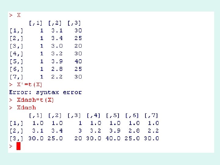
The model in matrix form is given by: We have already seen that Now calculate this for our example

R can be used to calculate X’X and the answer is:

To input the matrix in R use X=matrix(c(1, 1, 3. 4, 3. 0, 3. 4, 3. 9, 2. 8, 2. 2, 30, 25, 20, 30, 40, 25, 30), 7, 3) Number of rows Number of columns

Notice command for matrix multiplication

The inverse of X’X can also be obtained by using R

We also need to calculate X’Y Now

Notice that this is the same result as obtained previously using the lm result on R

So y = 0. 2138 + 0. 8984 x 1 + 0. 01745 x 2 + e

The “hat matrix” is given by

The fitted Y values are obtained by

Recall once more we are looking at the model

Compare with

Error Terms and Inference A useful result is : n : number of points k: number of explanatory variables

In addition we can show that: where s. e. (bi)= c (i+1) And c(i+1) is the (i+1)th diagonal element of

For our example:

was calculated as:

This means that c 11= 6. 683, c 22=0. 7600, c 33=0. 0053 Note that c 11 is associated with b 0, c 22 with b 1 and c 33 with b 2 We will calculate the standard error for b 1 This is 0. 7600 x 0. 2902 = 0. 2530

The value of ^b 1 is 0. 8984 Now carry out a hypothesis test. H 0: b 1 = 0 H 1: b 1 ≠ 0 The standard error of b 1 is 0. 2530

The test statistic is This calculates as (0. 8984 – 0)/0. 2530 = 3. 55

Ds…. . ………………. . . . t tables using 4 degrees of freedom give cut of point of 2. 776 for 2. 5%.

We therefore accept H 1. There is no evidence at the 5% level that b 1 is zero. The process can be repeated for the other b values and confidence intervals calculated in the usual way. CI for 2 - based on the 42 distribution of ((4 0. 08422)/11. 14 , (4 0. 08422)/0. 4844) i. e. (0. 030 , 0. 695)

The sum of squares of the residuals can also be calculated.