Multiple Linear Regression Learning Objectives Extend Simple Linear

Multiple Linear Regression Learning Objectives • Extend Simple Linear Regression concepts to regression with multiple explanatory variables • Apply the Matlab regression tools and interpret their output • Choose the variables to use in a multiple regression • Quantify the uncertainty of MLR predictions

Readings • • Kottegoda and Rosso, Chapter 6 (6. 2) Helsel and Hirsch, Chapters 9 and 11 Hastie, Tibshirani and Friedman, Chapter 3 Matlab Statistics Toolbox Users Guide, Chapter 6.

Multiple Linear Regression Model

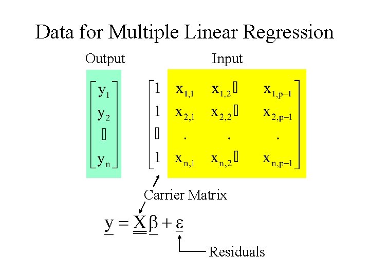
Data for Multiple Linear Regression Output Input Carrier Matrix Residuals

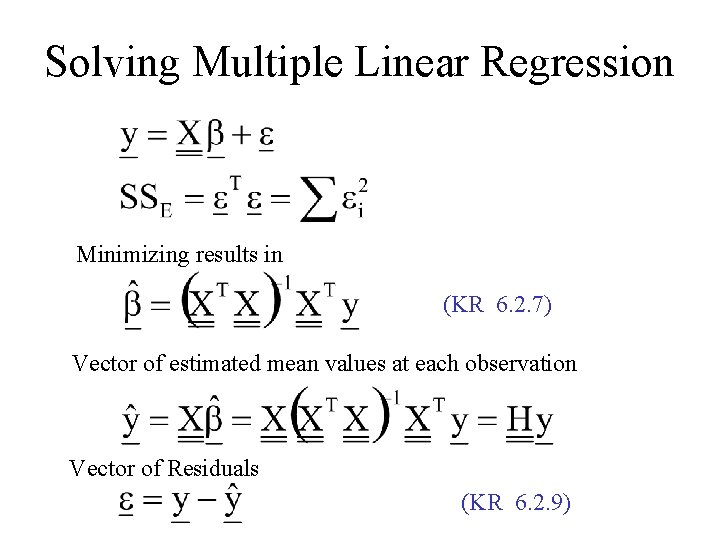
Solving Multiple Linear Regression Minimizing results in (KR 6. 2. 7) Vector of estimated mean values at each observation Vector of Residuals (KR 6. 2. 9)

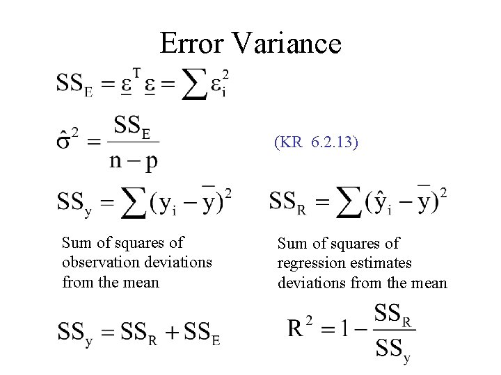
Error Variance (KR 6. 2. 13) Sum of squares of observation deviations from the mean Sum of squares of regression estimates deviations from the mean

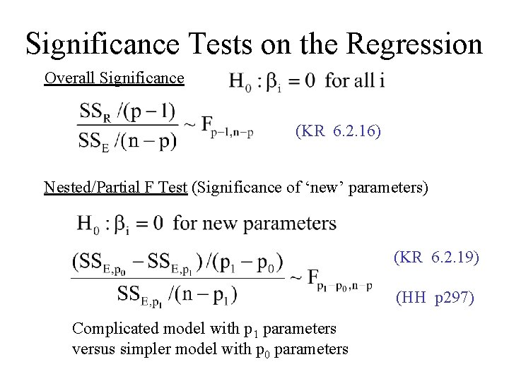
Significance Tests on the Regression Overall Significance (KR 6. 2. 16) Nested/Partial F Test (Significance of ‘new’ parameters) (KR 6. 2. 19) (HH p 297) Complicated model with p 1 parameters versus simpler model with p 0 parameters

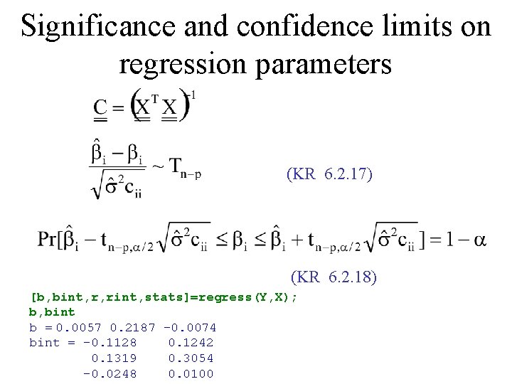
Significance and confidence limits on regression parameters (KR 6. 2. 17) (KR 6. 2. 18) [b, bint, r, rint, stats]=regress(Y, X); b, bint b = 0. 0057 0. 2187 -0. 0074 bint = -0. 1128 0. 1242 0. 1319 0. 3054 -0. 0248 0. 0100

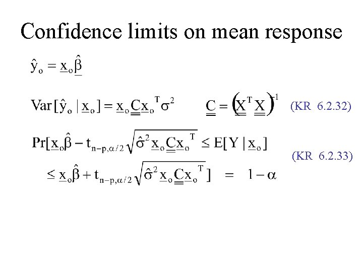
Confidence limits on mean response (KR 6. 2. 32) (KR 6. 2. 33)

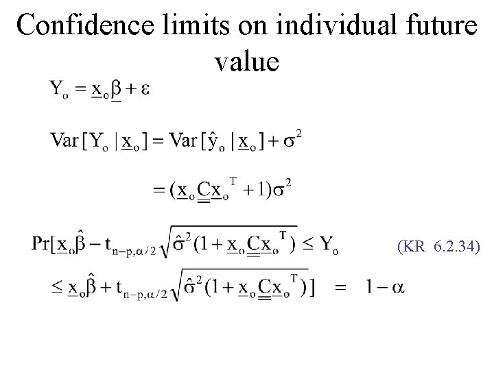
Confidence limits on individual future value (KR 6. 2. 34)

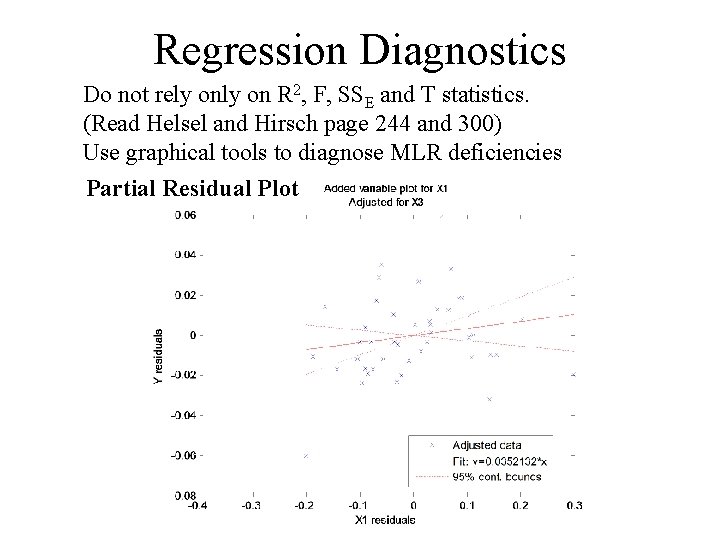
Regression Diagnostics Do not rely on R 2, F, SSE and T statistics. (Read Helsel and Hirsch page 244 and 300) Use graphical tools to diagnose MLR deficiencies Partial Residual Plot

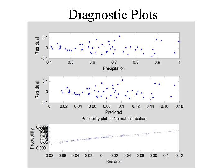
Diagnostic Plots

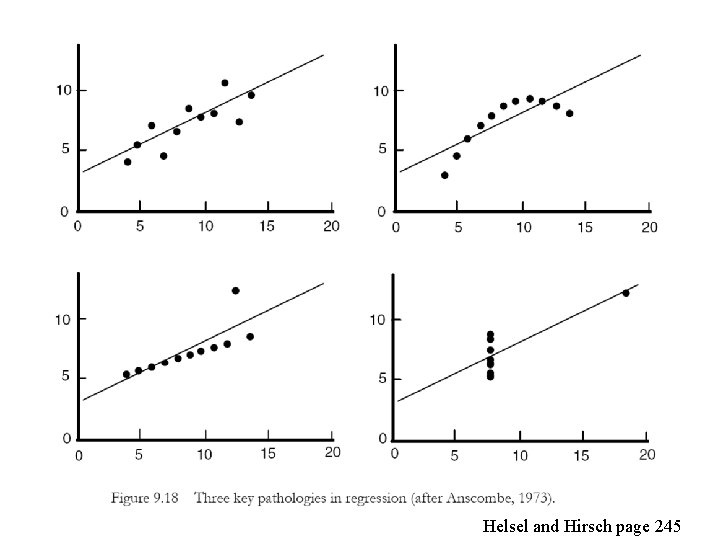
Helsel and Hirsch page 245

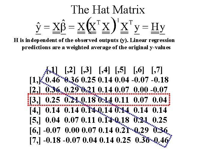
The Hat Matrix H is independent of the observed outputs (y). Linear regression predictions are a weighted average of the original y-values [, 1] [, 2] [, 3] [, 4] [, 5] [, 6] [, 7] [1, ] 0. 46 0. 36 0. 25 0. 14 0. 04 -0. 07 -0. 18 [2, ] 0. 36 0. 29 0. 21 0. 14 0. 07 0. 00 -0. 07 [3, ] 0. 25 0. 21 0. 18 0. 14 0. 11 0. 07 0. 04 [4, ] 0. 14 0. 14 [5, ] 0. 04 0. 07 0. 11 0. 14 0. 18 0. 21 0. 25 [6, ] -0. 07 0. 00 0. 07 0. 14 0. 21 0. 29 0. 36 [7, ] -0. 18 -0. 07 0. 04 0. 14 0. 25 0. 36 0. 46

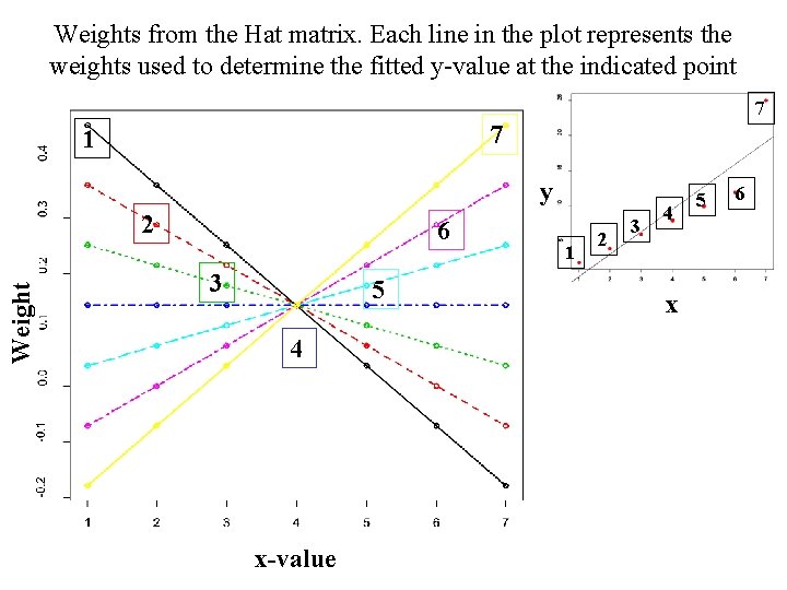
Weights from the Hat matrix. Each line in the plot represents the weights used to determine the fitted y-value at the indicated point 7 7 1 y Weight 2 6 3 5 4 x-value 1 2 3 4 x 5 6

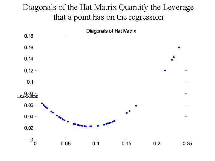
Diagonals of the Hat Matrix Quantify the Leverage that a point has on the regression

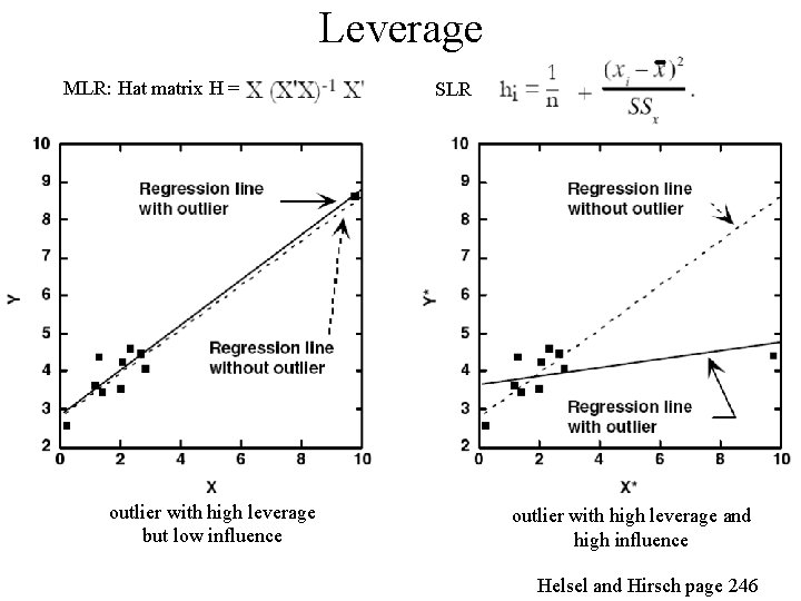
Leverage MLR: Hat matrix H = outlier with high leverage but low influence SLR outlier with high leverage and high influence Helsel and Hirsch page 246

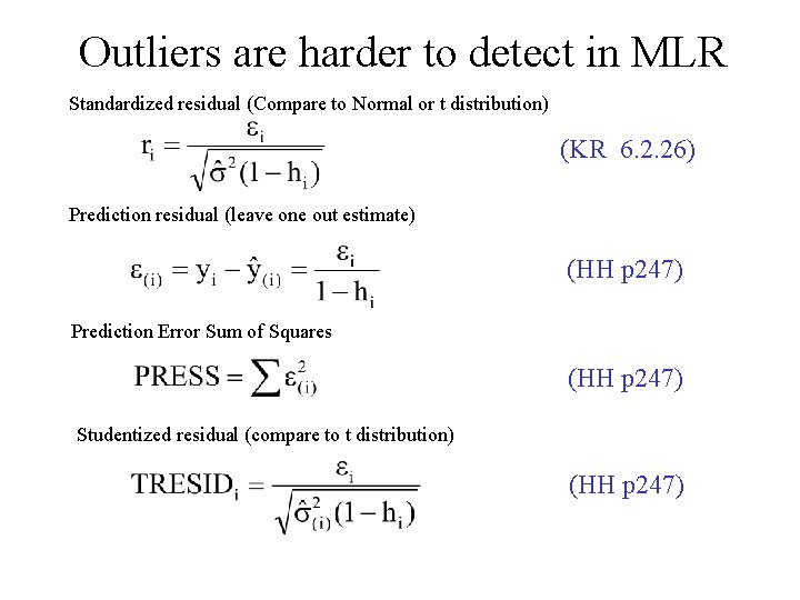
Outliers are harder to detect in MLR Standardized residual (Compare to Normal or t distribution) (KR 6. 2. 26) Prediction residual (leave one out estimate) (HH p 247) Prediction Error Sum of Squares (HH p 247) Studentized residual (compare to t distribution) (HH p 247)

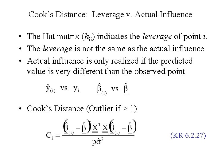
Cook’s Distance: Leverage v. Actual Influence • The Hat matrix (hii) indicates the leverage of point i. • The leverage is not the same as the actual influence. • Actual influence is only realized if the predicted value is very different than the observed point. • Cook’s Distance (Outlier if > 1) (KR 6. 2. 27)

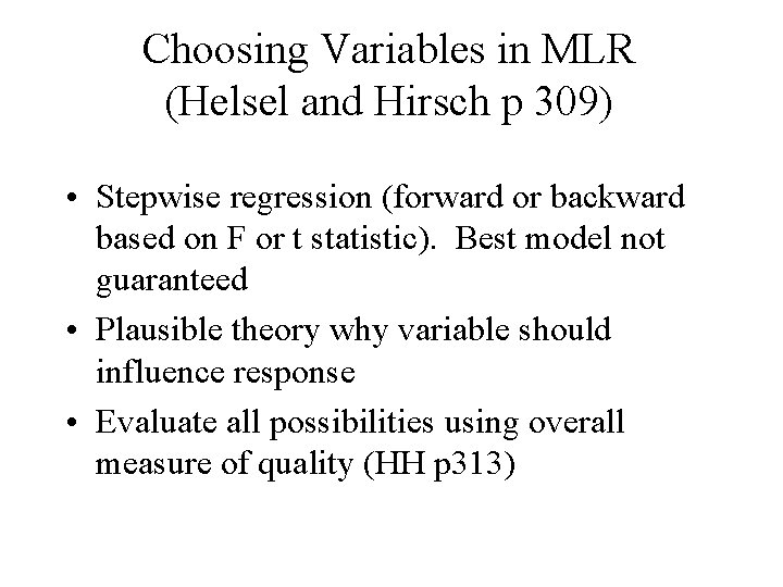
Choosing Variables in MLR (Helsel and Hirsch p 309) • Stepwise regression (forward or backward based on F or t statistic). Best model not guaranteed • Plausible theory why variable should influence response • Evaluate all possibilities using overall measure of quality (HH p 313)

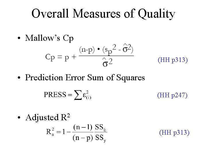
Overall Measures of Quality • Mallow’s Cp (HH p 313) • Prediction Error Sum of Squares (HH p 247) • Adjusted R 2 (HH p 313)