Multiple Linear Regression Introduction Introducing the General Linear

Multiple Linear Regression Introduction

Introducing the General

Linear Models • As noted by the General, the General Linear Model (GLM) can be used to relate one set of things (Ys) to another set of things (X). • It can also be used with only one set of things.

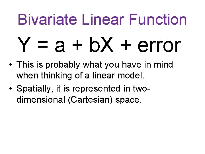
Bivariate Linear Function Y = a + b. X + error • This is probably what you have in mind when thinking of a linear model. • Spatially, it is represented in twodimensional (Cartesian) space.

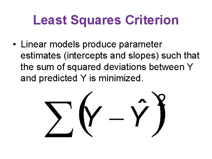
Least Squares Criterion • Linear models produce parameter estimates (intercepts and slopes) such that the sum of squared deviations between Y and predicted Y is minimized.

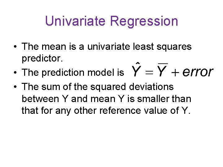
Univariate Regression • The mean is a univariate least squares predictor. • The prediction model is • The sum of the squared deviations between Y and mean Y is smaller than that for any other reference value of Y.

Multiple Regression • One continuous Y, two or more X variables. • X variables may be continuous or dichotomous • k groups may be represented by k-1 dichotomous dummy variables

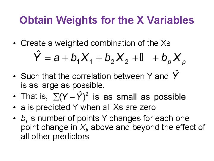
Obtain Weights for the X Variables • Create a weighted combination of the Xs • Such that the correlation between Y and is as large as possible. • That is, • a is predicted Y when all Xs are zero • bi is number of points Y changes for each one point change in Xi, above and beyond the effect of all other predictors.

Multiple R • The correlation between the Y variable and the predicted scores is R. • R 2 can be interpreted as a proportion of variance – the proportion of the variance in the Y scores that is explained by the weighted linear combination of the predictor scores. • Sample R 2 is biased – it overestimates the value of the corresponding population parameter.

Bias in Sample R 2 • Randomly select four scores. Randomly designate one as X for Case 1, one as Y for Case 1, one as X for Case 2, and one as Y for Case 2. • Plot the scores. You can fit them perfectly with a straight line. • Accordingly, sample R 2 = 1, even though the corresponding population parameter has value zero.

Shrunken R 2 • Reduces the bias in unadjusted R 2. • Bias will be greatest when the number of cases is small relative to the number of predictors. • Please run the SAS program Variables. Cases-R. • Draw a conclusion with respect to the relationship between R 2 and the number of cases and number of variables.

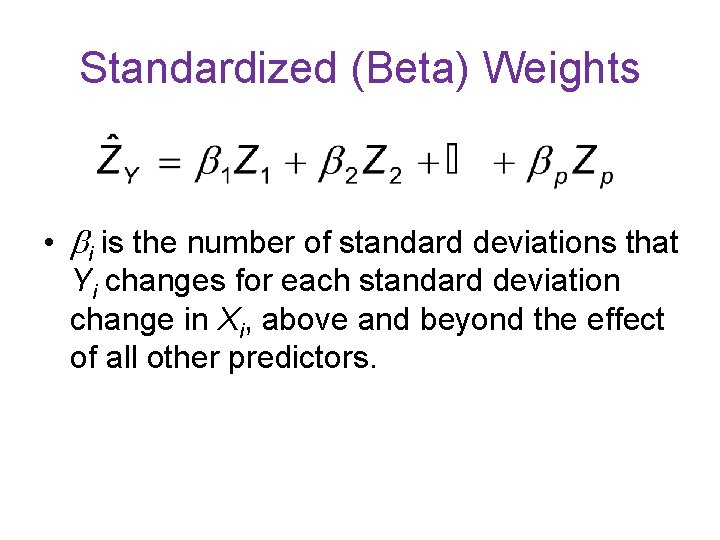
Standardized (Beta) Weights • i is the number of standard deviations that Yi changes for each standard deviation change in Xi, above and beyond the effect of all other predictors.

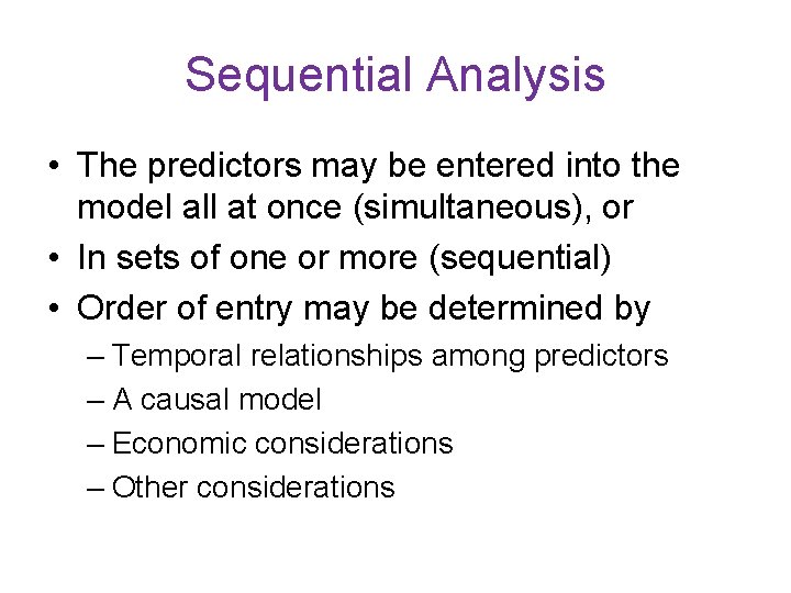
Sequential Analysis • The predictors may be entered into the model all at once (simultaneous), or • In sets of one or more (sequential) • Order of entry may be determined by – Temporal relationships among predictors – A causal model – Economic considerations – Other considerations

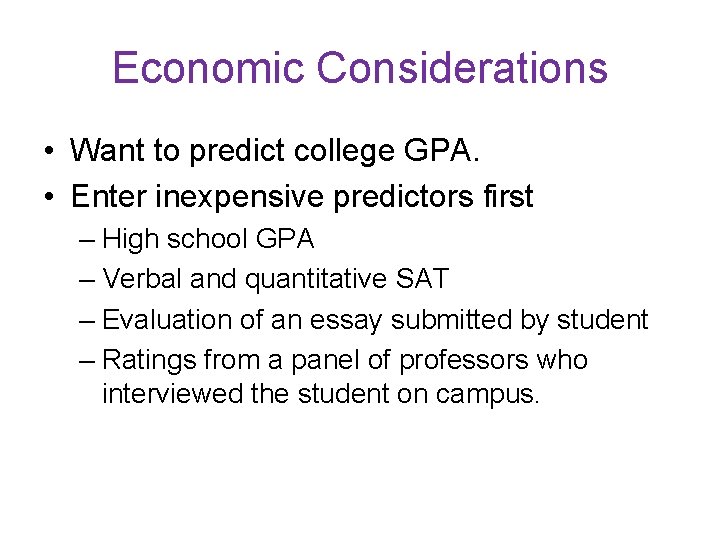
Economic Considerations • Want to predict college GPA. • Enter inexpensive predictors first – High school GPA – Verbal and quantitative SAT – Evaluation of an essay submitted by student – Ratings from a panel of professors who interviewed the student on campus.

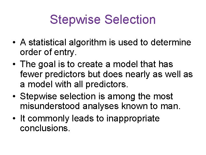
Stepwise Selection • A statistical algorithm is used to determine order of entry. • The goal is to create a model that has fewer predictors but does nearly as well as a model with all predictors. • Stepwise selection is among the most misunderstood analyses known to man. • It commonly leads to inappropriate conclusions.

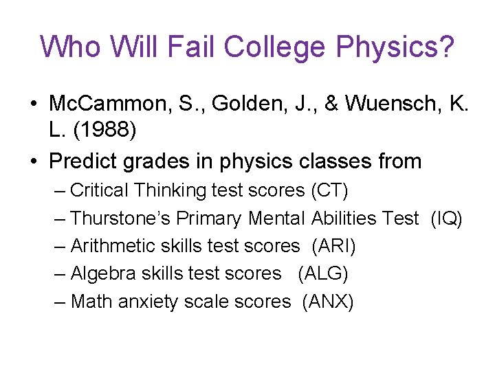
Who Will Fail College Physics? • Mc. Cammon, S. , Golden, J. , & Wuensch, K. L. (1988) • Predict grades in physics classes from – Critical Thinking test scores (CT) – Thurstone’s Primary Mental Abilities Test (IQ) – Arithmetic skills test scores (ARI) – Algebra skills test scores (ALG) – Math anxiety scale scores (ANX)

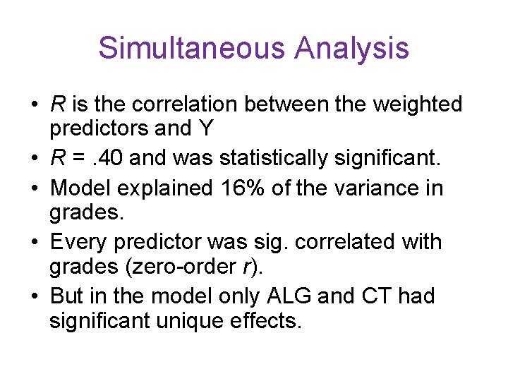
Simultaneous Analysis • R is the correlation between the weighted predictors and Y • R =. 40 and was statistically significant. • Model explained 16% of the variance in grades. • Every predictor was sig. correlated with grades (zero-order r). • But in the model only ALG and CT had significant unique effects.

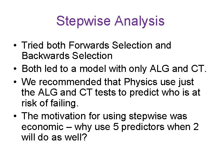
Stepwise Analysis • Tried both Forwards Selection and Backwards Selection • Both led to a model with only ALG and CT. • We recommended that Physics use just the ALG and CT tests to predict who is at risk of failing. • The motivation for using stepwise was economic – why use 5 predictors when 2 will do as well?

Does Sex Matter? • Mc. Cammon insisted that I address this issue. • Means and variances differed little between the sexes. • Just to please Mc. Cammon, I did the analysis separately for men and women.

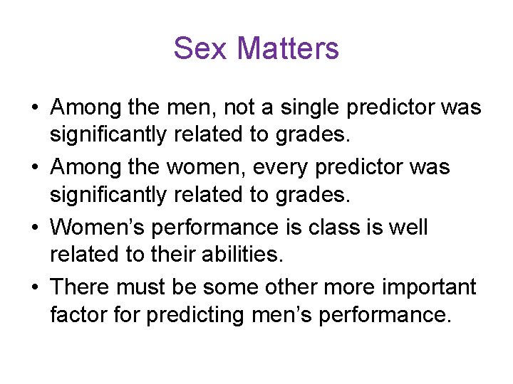
Sex Matters • Among the men, not a single predictor was significantly related to grades. • Among the women, every predictor was significantly related to grades. • Women’s performance is class is well related to their abilities. • There must be some other more important factor for predicting men’s performance.

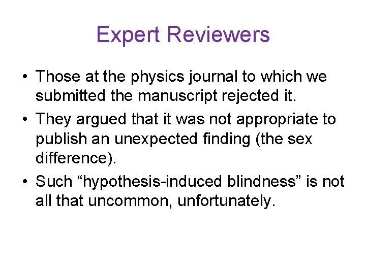
Expert Reviewers • Those at the physics journal to which we submitted the manuscript rejected it. • They argued that it was not appropriate to publish an unexpected finding (the sex difference). • Such “hypothesis-induced blindness” is not all that uncommon, unfortunately.

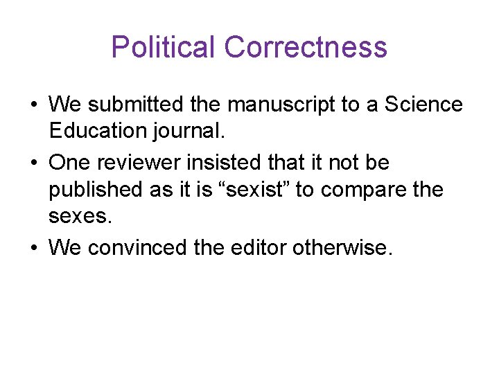
Political Correctness • We submitted the manuscript to a Science Education journal. • One reviewer insisted that it not be published as it is “sexist” to compare the sexes. • We convinced the editor otherwise.