MULTIPLE LINEAR REGRESSION INTERPRETATION OF COEFFICIENTS The Multiple

MULTIPLE LINEAR REGRESSION INTERPRETATION OF COEFFICIENTS

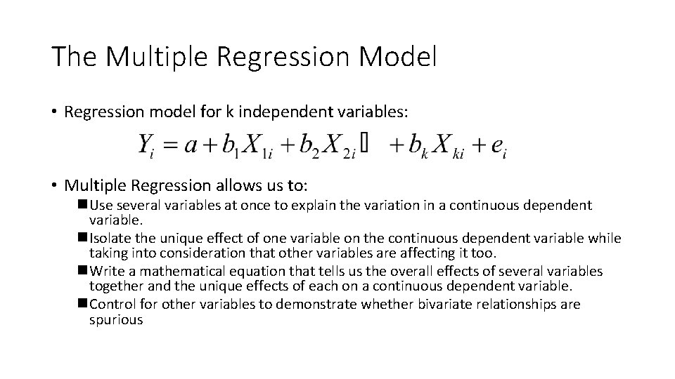
The Multiple Regression Model • Regression model for k independent variables: • Multiple Regression allows us to: n Use several variables at once to explain the variation in a continuous dependent variable. n Isolate the unique effect of one variable on the continuous dependent variable while taking into consideration that other variables are affecting it too. n Write a mathematical equation that tells us the overall effects of several variables together and the unique effects of each on a continuous dependent variable. n Control for other variables to demonstrate whether bivariate relationships are spurious

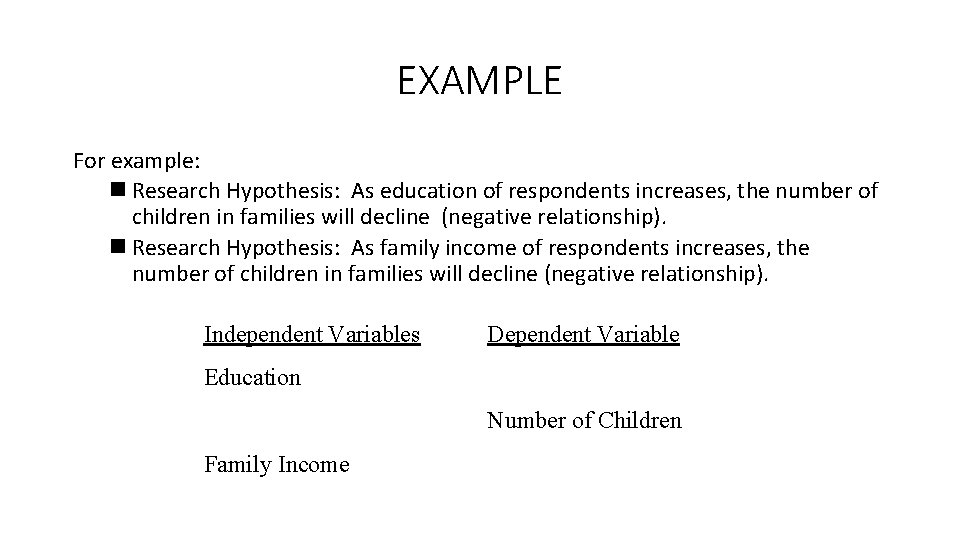
EXAMPLE For example: n Research Hypothesis: As education of respondents increases, the number of children in families will decline (negative relationship). n Research Hypothesis: As family income of respondents increases, the number of children in families will decline (negative relationship). Independent Variables Dependent Variable Education Number of Children Family Income

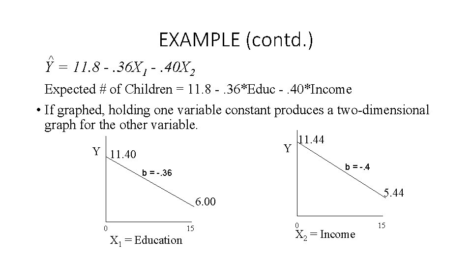
EXAMPLE (contd. ) Y = 11. 8 -. 36 X 1 -. 40 X 2 Expected # of Children = 11. 8 -. 36*Educ -. 40*Income • If graphed, holding one variable constant produces a two-dimensional graph for the other variable. Y Y 11. 40 11. 44 b = -. 36 5. 44 6. 00 0 15 X 1 = Education 0 X 2 = Income 15

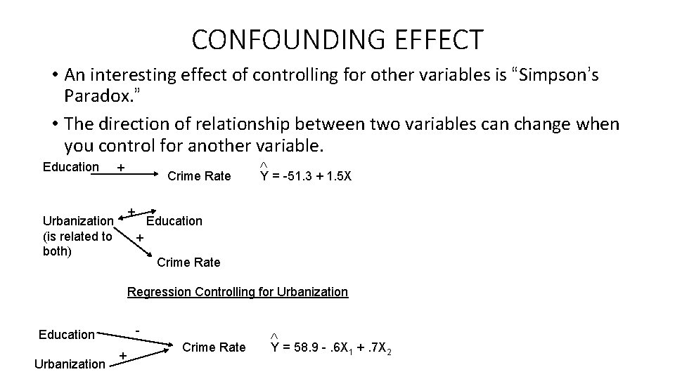
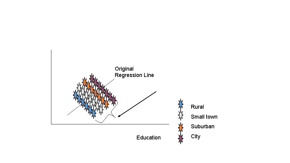
CONFOUNDING EFFECT • An interesting effect of controlling for other variables is “Simpson’s Paradox. ” • The direction of relationship between two variables can change when you control for another variable. Education + Crime Rate + Urbanization (is related to both) Y = -51. 3 + 1. 5 X Education + Crime Rate Regression Controlling for Urbanization - Education Urbanization + Crime Rate Y = 58. 9 -. 6 X 1 +. 7 X 2

Original Regression Line Rural Small town Suburban Education City

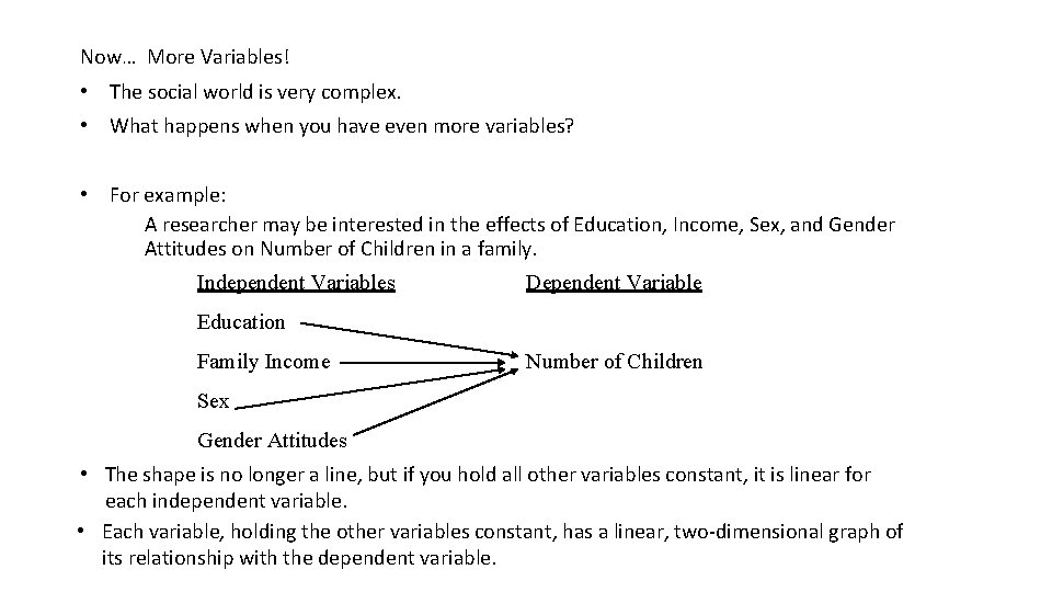
Now… More Variables! • The social world is very complex. • What happens when you have even more variables? • For example: A researcher may be interested in the effects of Education, Income, Sex, and Gender Attitudes on Number of Children in a family. Independent Variables Dependent Variable Education Family Income Number of Children Sex Gender Attitudes • The shape is no longer a line, but if you hold all other variables constant, it is linear for each independent variable. • Each variable, holding the other variables constant, has a linear, two-dimensional graph of its relationship with the dependent variable.

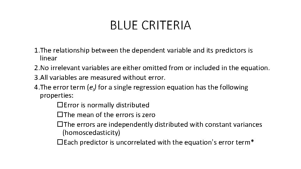
The BLUE Regression Criteria • Regression forces a best-fitting model onto data. If the model is appropriate for the data, regression should be used. • Criteria for determining whether a regression model is appropriate for the data are nicknamed “BLUE” for best linear unbiased estimate. • Violating the BLUE assumptions may result in biased estimates or incorrect significance tests. (However, OLS is robust to most violations. )

BLUE CRITERIA 1. The relationship between the dependent variable and its predictors is linear 2. No irrelevant variables are either omitted from or included in the equation. 3. All variables are measured without error. 4. The error term (ei) for a single regression equation has the following properties: o. Error is normally distributed o. The mean of the errors is zero o. The errors are independently distributed with constant variances (homoscedasticity) o. Each predictor is uncorrelated with the equation’s error term*

DUMMY VARIABLES • They are simply dichotomous variables that are entered into regression. They have 0 – 1 coding where 0 = absence of something and 1 = presence of something. E. g. , Female (0=M; 1=F) or Southern (0=Non-Southern; 1=Southern). • Dummy Variables are especially nice because they allow us to use nominal variables in regression. • A nominal variable has no rank or order, rendering the numerical coding scheme useless for regression.

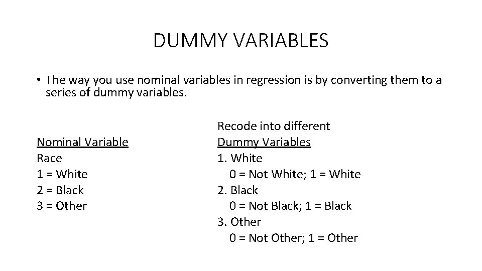
DUMMY VARIABLES • The way you use nominal variables in regression is by converting them to a series of dummy variables. Nominal Variable Race 1 = White 2 = Black 3 = Other Recode into different Dummy Variables 1. White 0 = Not White; 1 = White 2. Black 0 = Not Black; 1 = Black 3. Other 0 = Not Other; 1 = Other

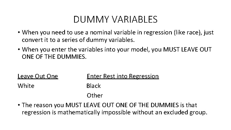
DUMMY VARIABLES • When you need to use a nominal variable in regression (like race), just convert it to a series of dummy variables. • When you enter the variables into your model, you MUST LEAVE OUT ONE OF THE DUMMIES. Leave Out One White Enter Rest into Regression Black Other • The reason you MUST LEAVE OUT ONE OF THE DUMMIES is that regression is mathematically impossible without an excluded group.

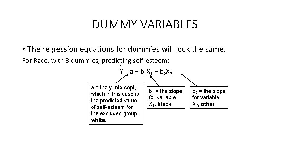
DUMMY VARIABLES • The regression equations for dummies will look the same. For Race, with 3 dummies, predicting self-esteem: Y = a + b 1 X 1 + b 2 X 2 a = the y-intercept, which in this case is the predicted value of self-esteem for the excluded group, white. b 1 = the slope for variable X 1, black b 2 = the slope for variable X 2, other

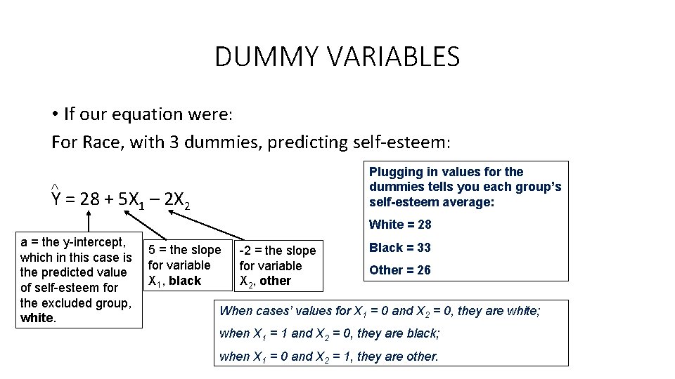
DUMMY VARIABLES • If our equation were: For Race, with 3 dummies, predicting self-esteem: Plugging in values for the dummies tells you each group’s self-esteem average: Y = 28 + 5 X 1 – 2 X 2 White = 28 a = the y-intercept, which in this case is the predicted value of self-esteem for the excluded group, white. 5 = the slope for variable X 1, black -2 = the slope for variable X 2, other Black = 33 Other = 26 When cases’ values for X 1 = 0 and X 2 = 0, they are white; when X 1 = 1 and X 2 = 0, they are black; when X 1 = 0 and X 2 = 1, they are other.

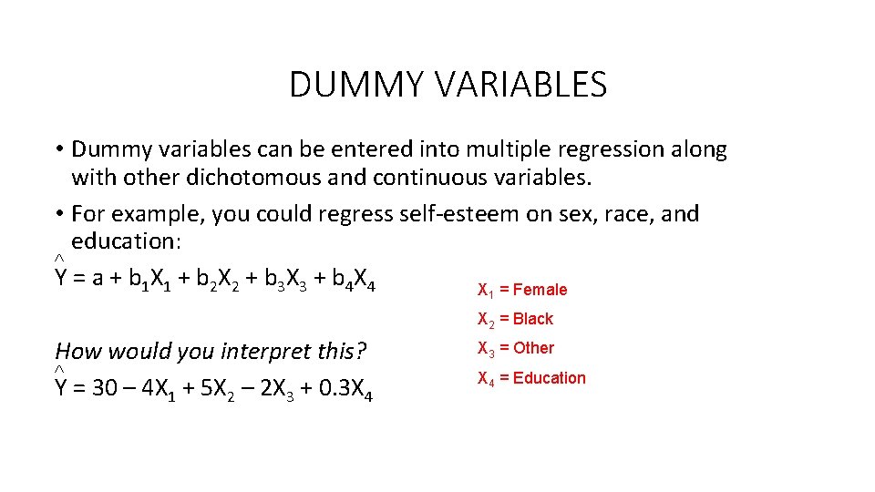
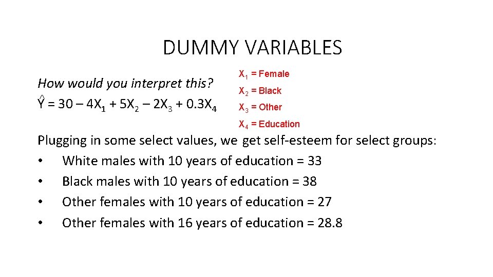
DUMMY VARIABLES • Dummy variables can be entered into multiple regression along with other dichotomous and continuous variables. • For example, you could regress self-esteem on sex, race, and education: Y = a + b 1 X 1 + b 2 X 2 + b 3 X 3 + b 4 X = Female 1 X 2 = Black How would you interpret this? Y = 30 – 4 X 1 + 5 X 2 – 2 X 3 + 0. 3 X 4 X 3 = Other X 4 = Education

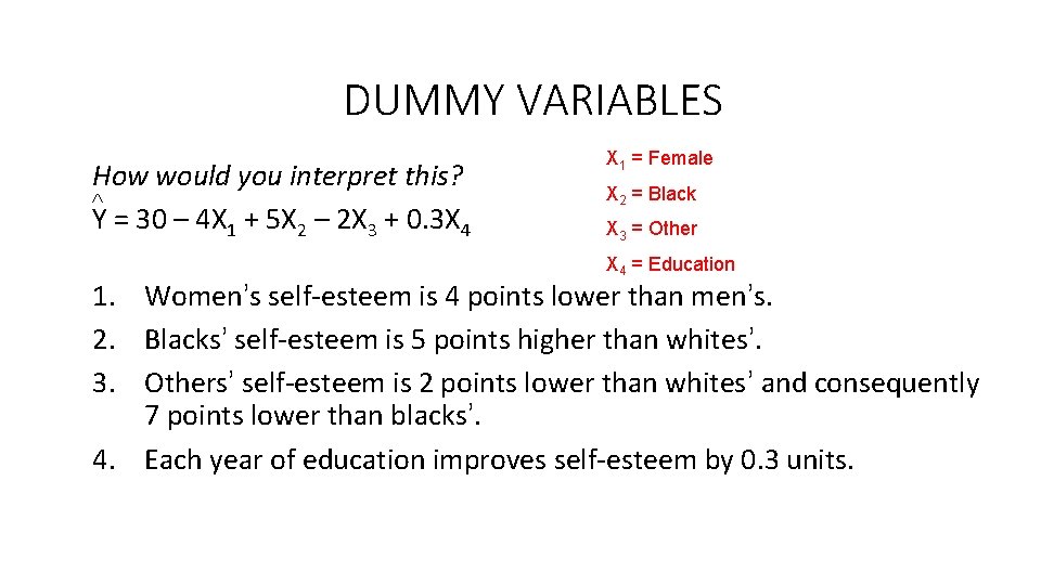
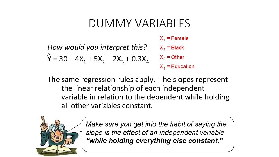
DUMMY VARIABLES How would you interpret this? Y = 30 – 4 X 1 + 5 X 2 – 2 X 3 + 0. 3 X 4 X 1 = Female X 2 = Black X 3 = Other X 4 = Education 1. Women’s self-esteem is 4 points lower than men’s. 2. Blacks’ self-esteem is 5 points higher than whites’. 3. Others’ self-esteem is 2 points lower than whites’ and consequently 7 points lower than blacks’. 4. Each year of education improves self-esteem by 0. 3 units.

DUMMY VARIABLES How would you interpret this? Y = 30 – 4 X 1 + 5 X 2 – 2 X 3 + 0. 3 X 4 X 1 = Female X 2 = Black X 3 = Other X 4 = Education Plugging in some select values, we get self-esteem for select groups: • White males with 10 years of education = 33 • Black males with 10 years of education = 38 • Other females with 10 years of education = 27 • Other females with 16 years of education = 28. 8

DUMMY VARIABLES How would you interpret this? Y = 30 – 4 X 1 + 5 X 2 – 2 X 3 + 0. 3 X 4 X 1 = Female X 2 = Black X 3 = Other X 4 = Education The same regression rules apply. The slopes represent the linear relationship of each independent variable in relation to the dependent while holding all other variables constant. Make sure you get into the habit of saying the slope is the effect of an independent variable “while holding everything else constant. ”

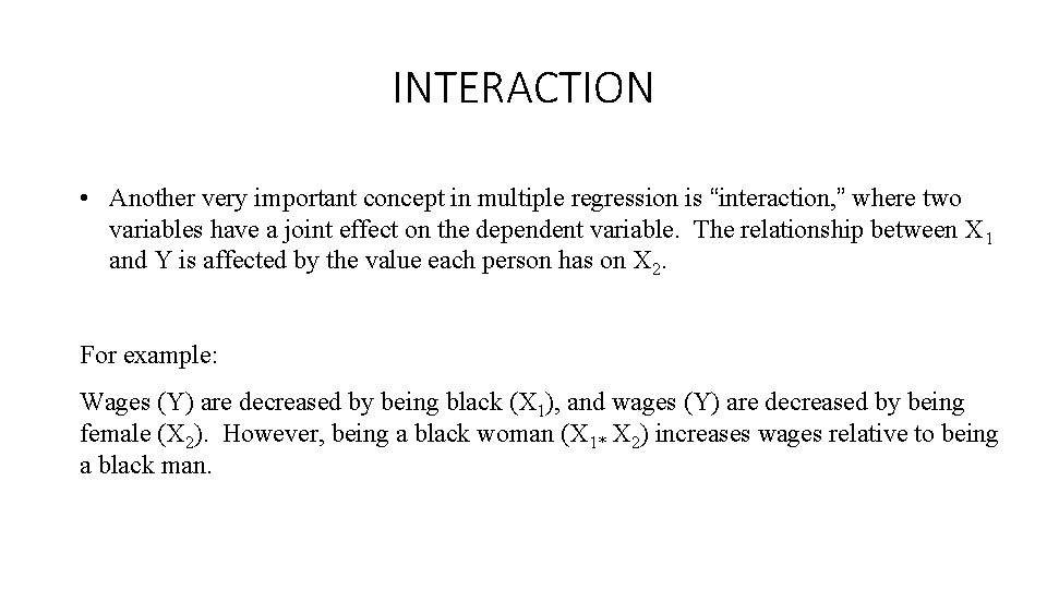
INTERACTION • Another very important concept in multiple regression is “interaction, ” where two variables have a joint effect on the dependent variable. The relationship between X 1 and Y is affected by the value each person has on X 2. For example: Wages (Y) are decreased by being black (X 1), and wages (Y) are decreased by being female (X 2). However, being a black woman (X 1* X 2) increases wages relative to being a black man.

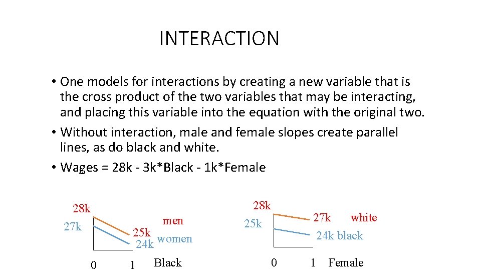
INTERACTION • One models for interactions by creating a new variable that is the cross product of the two variables that may be interacting, and placing this variable into the equation with the original two. • Without interaction, male and female slopes create parallel lines, as do black and white. • Wages = 28 k - 3 k*Black - 1 k*Female ^ 28 k 27 k 0 men 25 k women 24 k Black 1 28 k 25 k 27 k white 24 k black 0 1 Female

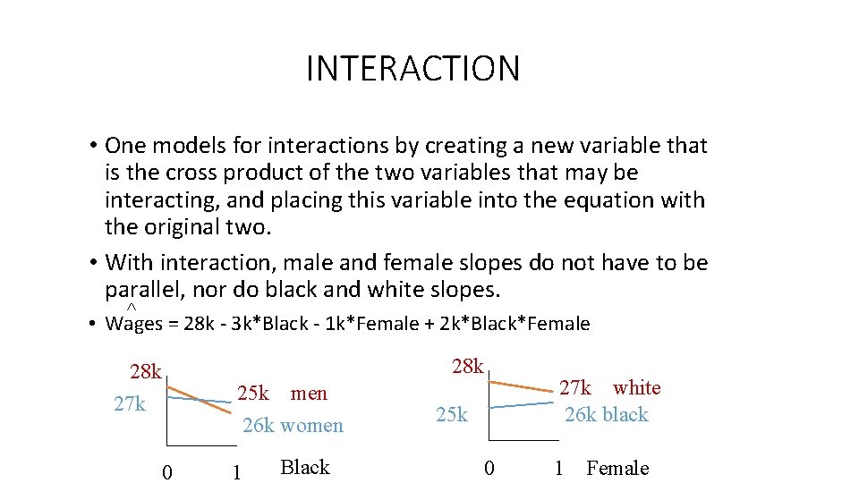
INTERACTION • One models for interactions by creating a new variable that is the cross product of the two variables that may be interacting, and placing this variable into the equation with the original two. • With interaction, male and female slopes do not have to be parallel, nor do black and white slopes. ^ • Wages = 28 k - 3 k*Black - 1 k*Female + 2 k*Black*Female 28 k 27 k 25 k men 26 k women 0 1 Black 27 k white 26 k black 25 k 0 1 Female

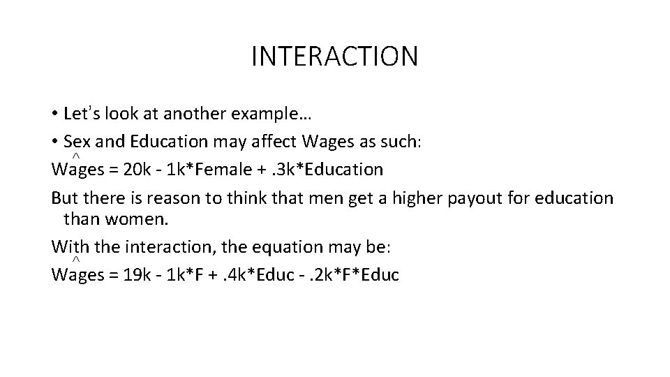
INTERACTION • Let’s look at another example… • Sex and Education may affect Wages as such: ^ Wages = 20 k - 1 k*Female +. 3 k*Education But there is reason to think that men get a higher payout for education than women. With the interaction, the equation may be: ^ Wages = 19 k - 1 k*F +. 4 k*Educ -. 2 k*F*Educ

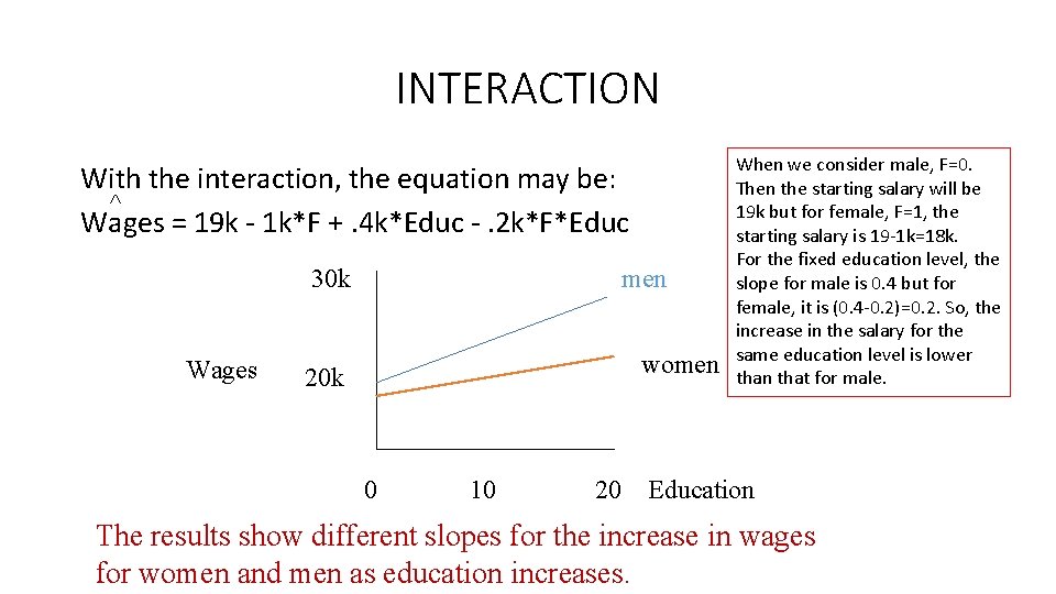
INTERACTION With the interaction, the equation may be: ^ Wages = 19 k - 1 k*F +. 4 k*Educ -. 2 k*F*Educ 30 k Wages men women 20 k 0 10 20 When we consider male, F=0. Then the starting salary will be 19 k but for female, F=1, the starting salary is 19 -1 k=18 k. For the fixed education level, the slope for male is 0. 4 but for female, it is (0. 4 -0. 2)=0. 2. So, the increase in the salary for the same education level is lower than that for male. Education The results show different slopes for the increase in wages for women and men as education increases.

INTERACTION • When one suspects that interactions may be occurring in the social world, it is appropriate to test for them. • To test for an interaction, enter an “interaction term” into the regression along with the original two variables. • If the interaction slope is significant, you have interaction in the population. Report that! • If the slope is not significant, remove the interaction term from your model.

Interaction Terms • Question: What if you suspect that a variable has a totally different slope for two different sub-groups in your data? • Example: Income and Happiness • Perhaps men are more materialistic -- an extra dollar increases their happiness a lot • If women are less materialistic, each dollar has a smaller effect on income (compared to men) • Issue isn’t men = “more” or “less” than women • Rather, the slope of a variable (income) differs across groups • Again, we want to specify a different regression line for each group • We want lines with different slopes, not parallel lines that are higher or lower.

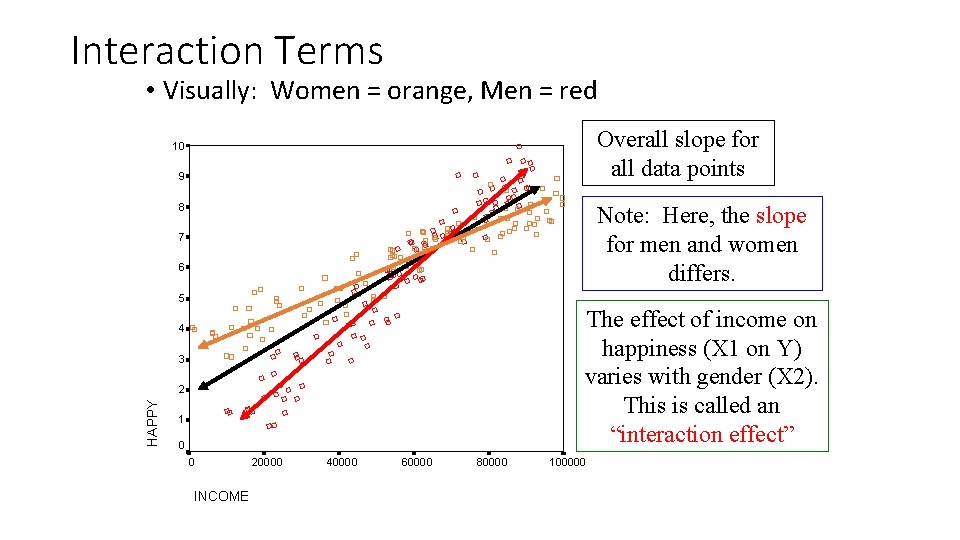
Interaction Terms • Visually: Women = orange, Men = red Overall slope for all data points 10 9 8 Note: Here, the slope for men and women differs. 7 6 5 The effect of income on happiness (X 1 on Y) varies with gender (X 2). This is called an “interaction effect” 4 3 HAPPY 2 1 0 0 INCOME 20000 40000 60000 80000 100000

Interaction Terms • Examples of interaction: • Effect of education on income may interact with type of school attended (public vs. private) • Private schooling has bigger effect on income • Effect of aspirations on educational attainment interacts with poverty • Aspirations matter less if you don’t have money to pay for college • Question: Can you think of examples of two variables that might interact? • Either from your final project? Or anything else?

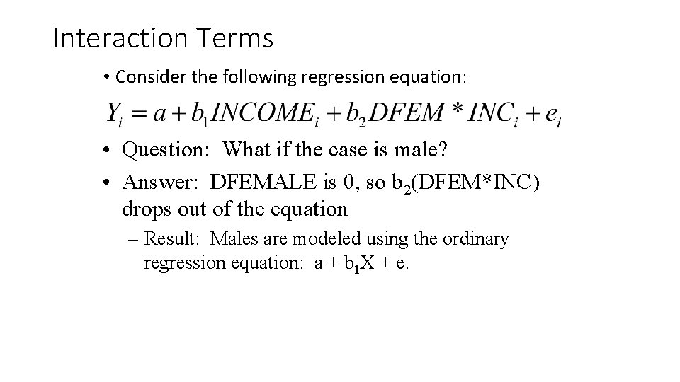
Interaction Terms • Interaction effects: Differences in the relationship (slope) between two variables for each category of a third variable • Option #1: Analyze each group separately • Look for different sized slope in each group • Option #2: Multiply the two variables of interest: (DFEMALE, INCOME) to create a new variable • Called: DFEMALE*INCOME • Add that variable to the multiple regression model.

Interaction Terms • Consider the following regression equation: • Question: What if the case is male? • Answer: DFEMALE is 0, so b 2(DFEM*INC) drops out of the equation – Result: Males are modeled using the ordinary regression equation: a + b 1 X + e.

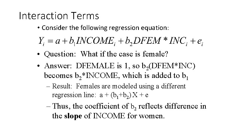
Interaction Terms • Consider the following regression equation: • Question: What if the case is female? • Answer: DFEMALE is 1, so b 2(DFEM*INC) becomes b 2*INCOME, which is added to b 1 – Result: Females are modeled using a different regression line: a + (b 1+b 2) X + e – Thus, the coefficient of b 2 reflects difference in the slope of INCOME for women.

Interpreting Interaction Terms • Interpreting interaction terms: • A positive b for DFEMALE*INCOME indicates the slope for income is higher for women vs. men • A negative effect indicates the slope is lower • Size of coefficient indicates actual difference in slope • Example: DFEMALE*INCOME. Observed b’s: • Income: b =. 5 • DFEMALE * INCOME: b = -. 2 • Interpretation: Slope is. 5 for men, . 3 for women.

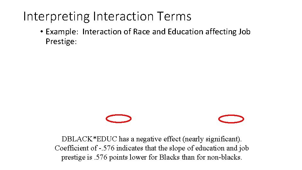
Interpreting Interaction Terms • Example: Interaction of Race and Education affecting Job Prestige: DBLACK*EDUC has a negative effect (nearly significant). Coefficient of -. 576 indicates that the slope of education and job prestige is. 576 points lower for Blacks than for non-blacks.

Continuous Interaction Terms • Two continuous variables can also interact • Example: Effect of education and income on happiness • Perhaps highly educated people are less materialistic • As education increases, the slope between income and happiness would decrease • Simply multiply Education and Income to create the interaction term “EDUCATION*INCOME” • And add it to the model.

Interpreting Interaction Terms • How do you interpret continuous variable interactions? • Example: EDUCATION*INCOME: Coefficient = 2. 0 • Answer: For each unit change in education, the slope of income vs. happiness increases by 2 • Note: coefficient is symmetrical: For each unit change in income, education slope increases by 2 • Dummy interactions effectively estimate 2 slopes: one for each group • Continuous interactions result in many slopes: Each value of education*income yields a different slope. =

Interpreting Interaction Terms • Interaction terms alters the interpretation of “main effect” coefficients • Including “EDUC*INCOME changes the interpretation of EDUC and of INCOME • Specifically, coefficient for EDUC represents slope of EDUC when INCOME = 0 • Likewise, INCOME shows slope when AGE=0 • Thus, main effects are like “baseline” slopes • And, the interaction effect coefficient shows how the slope grows (or shrinks) for a given unit change.

Dummy Interactions • It is also possible to construct interaction terms based on two dummy variables • Instead of a “slope” interaction, dummy interactions show difference in constants • Constant (not slope) differs across values of a third variable Example: Effect of race on school success varies by gender • African Americans do less well in school; but the difference is much larger for black males.

Dummy Interactions • Strategy for dummy interaction is the same: Multiply both variables Example: • Multiply DBLACK, DMALE to create DBLACK*DMALE • Then, include all 3 variables in the model • Effect of DBLACK*DMALE reflects difference in constant (level) for black males, compared to white males and black females • You would observe a negative coefficient, indicating that black males fare worse in schools than black females or white males.

Interaction Terms Comments: 1. If you make an interaction you should also include the component variables in the model: A model with “DFEMALE * INCOME” should also include DFEMALE and INCOME There are rare exceptions. But when in doubt, include them 2. Sometimes interaction terms are highly correlated with its components • That can cause problems (multicollinearity). 3. Make sure you have enough cases in each group for your interaction terms • Interaction terms involve estimating slopes based on sub-groups in your data (e. g. , black females). • If you there are hardly any black females in the dataset, you can have problems.

Interaction Terms 4. Interaction terms are confusing at first… but they are VERY important Example: Race, class, gender. Most sociologists argue that they operate interactively The experience of black lower-class females is different from black upper-class females or white lower-class females Interaction terms are a powerful way of identifying such intersections in quantitative data In short: Make the effort to consider how variables interact… it is a very useful way of thinking.

Standardized Coefficients • Sometimes you want to know whether one variable has a larger impact on your dependent variable than another. • If your variables have different units of measure, it is hard to compare their effects. • For example, if wages go up one thousand dollars for each year of education, is that a greater effect than if wages go up five hundred dollars for each year increase in age.

Standardized Coefficients • So which is better for increasing wages, education or aging? • One thing you can do is “standardize” your slopes so that you can compare the standard deviation increase in your dependent variable for each standard deviation increase in your independent variables. • You might find that Wages go up 0. 3 standard deviations for each standard deviation increase in education, but 0. 4 standard deviations for each standard deviation increase in age.

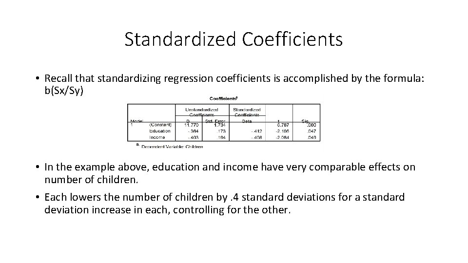
Standardized Coefficients • Recall that standardizing regression coefficients is accomplished by the formula: b(Sx/Sy) • In the example above, education and income have very comparable effects on number of children. • Each lowers the number of children by. 4 standard deviations for a standard deviation increase in each, controlling for the other.

Standardized Coefficients • One last note of caution. . . n. It does not make sense to standardize slopes for dichotomous variables. n. It makes no sense to refer to standard deviation increases in sex, or in race-these are either 0 or they are 1 only.