Multiple and complex regression Extensions of simple linear

Multiple and complex regression

Extensions of simple linear regression • Multiple regression models: predictor variables are continuous • Analysis of variance: predictor variables are categorical (grouping variables), • But… general linear models can include both continuous and categorical predictors

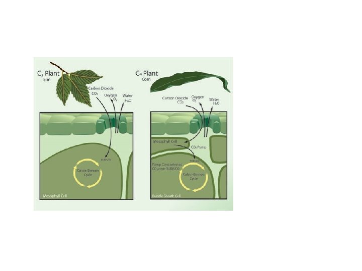
Relative abundance of C 3 and C 4 plants • Paruelo & Lauenroth (1996) • Geographic distribution and the effects of climate variables on the relative abundance of a number of plant functional types (PFTs): shrubs, forbs, succulents, C 3 grasses and C 4 grasses.

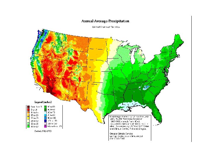
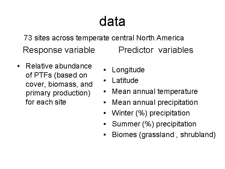
data 73 sites across temperate central North America Response variable • Relative abundance of PTFs (based on cover, biomass, and primary production) for each site Predictor variables • • Longitude Latitude Mean annual temperature Mean annual precipitation Winter (%) precipitation Summer (%) precipitation Biomes (grassland , shrubland)

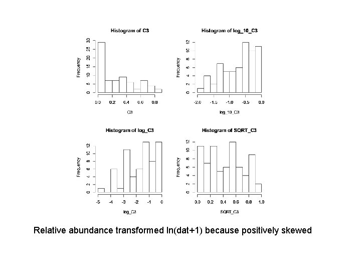
Relative abundance transformed ln(dat+1) because positively skewed

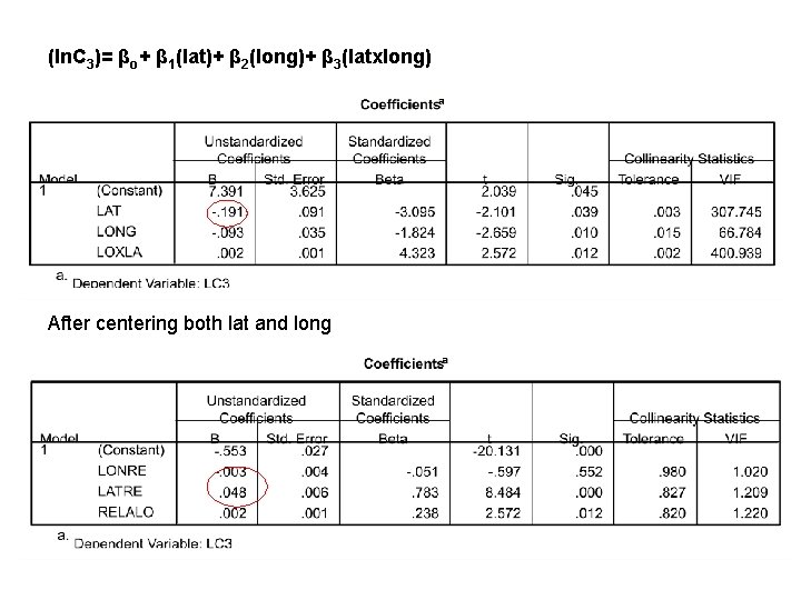
Collinearity • Causes computational problems because it makes the determinant of the matrix of X -variables close to zero and matrix inversion basically involves dividing by the determinant (very sensitive to small differences in the numbers) • Standard errors of the estimated regression slopes are inflated

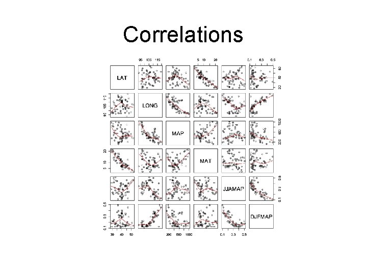
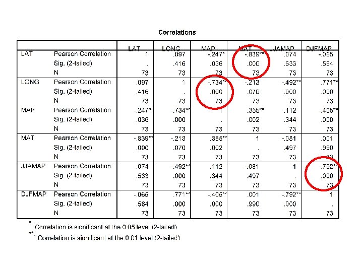
Detecting collinearlity • Check tolerance values • Plot the variables • Examine a matrix of correlation coefficients between predictor variables

Dealing with collinearity • Omit predictor variables if they are highly correlated with other predictor variables that remain in the model

Correlations

(ln. C 3)= βo+ β 1(lat)+ β 2(long)+ β 3(latxlong) After centering both lat and long

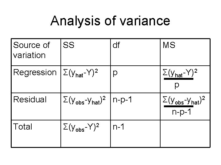
Analysis of variance Source of variation SS Regression Σ(yhat-Y)2 df MS p Σ(yhat-Y)2 p Residual Σ(yobs-yhat)2 n-p-1 Total Σ(yobs-Y)2 n-1 Σ(yobs-yhat)2 n-p-1

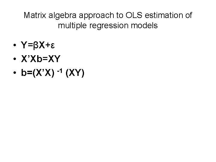
Matrix algebra approach to OLS estimation of multiple regression models • Y=βX+ε • X’Xb=XY • b=(X’X) -1 (XY)

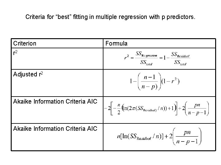
Criteria for “best” fitting in multiple regression with p predictors. Criterion r 2 Adjusted r 2 Akaike Information Criteria AIC Formula

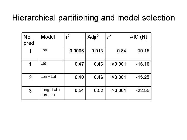
Hierarchical partitioning and model selection No pred Model r 2 Adjr 2 P AIC (R) 1 Lon 0. 0006 -0. 013 0. 84 30. 15 1 Lat 0. 47 0. 46 >0. 001 -16. 16 2 Lon + Lat 0. 48 0. 46 >0. 001 -15. 25 3 Long +Lat + Lon x Lat 0. 54 0. 52 >0. 001 -22. 55

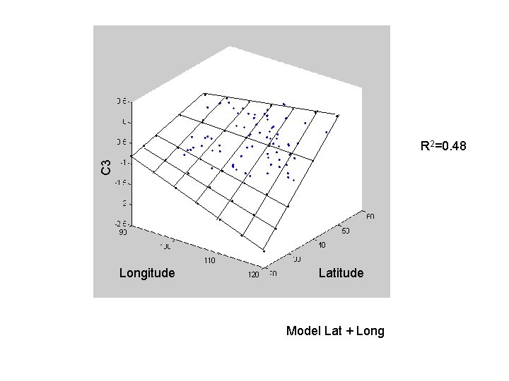
C 3 R 2=0. 48 Longitude Latitude Model Lat + Long

45 Lat 35 Lat Model Lat * Long

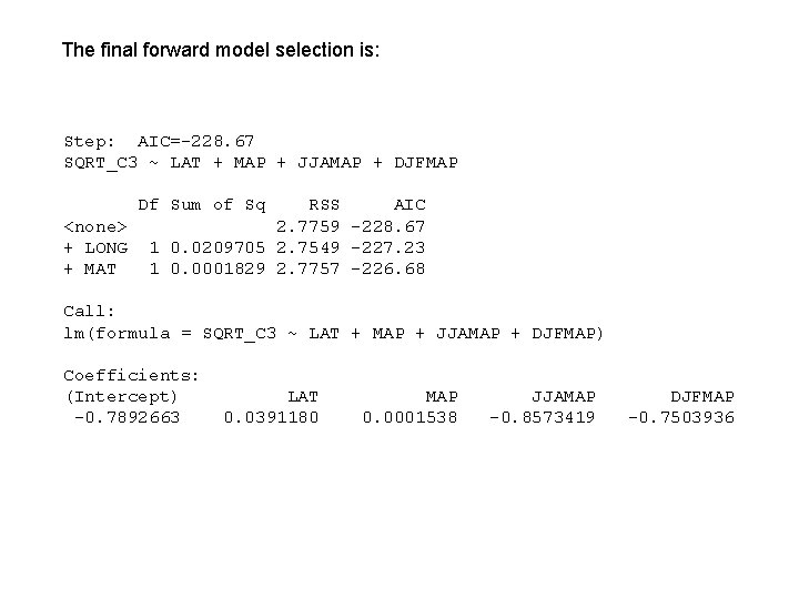
The final forward model selection is: Step: AIC=-228. 67 SQRT_C 3 ~ LAT + MAP + JJAMAP + DJFMAP Df Sum of Sq <none> + LONG + MAT RSS AIC 2. 7759 -228. 67 1 0. 0209705 2. 7549 -227. 23 1 0. 0001829 2. 7757 -226. 68 Call: lm(formula = SQRT_C 3 ~ LAT + MAP + JJAMAP + DJFMAP) Coefficients: (Intercept) -0. 7892663 LAT 0. 0391180 MAP 0. 0001538 JJAMAP -0. 8573419 DJFMAP -0. 7503936

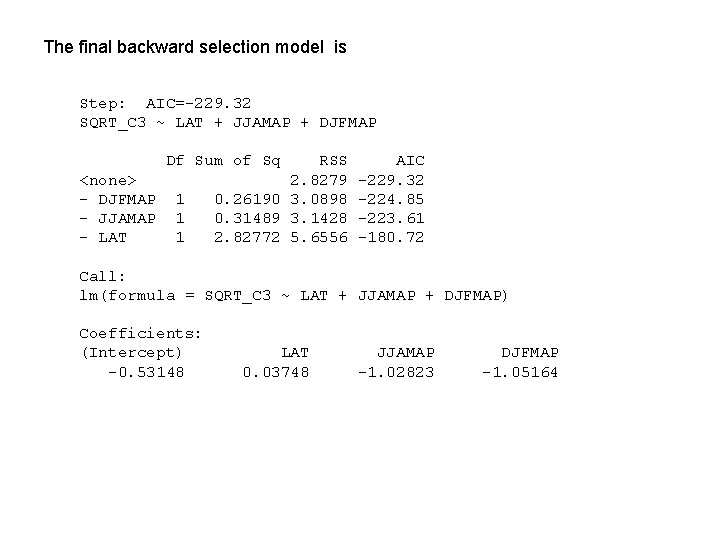
The final backward selection model is Step: AIC=-229. 32 SQRT_C 3 ~ LAT + JJAMAP + DJFMAP Df Sum of Sq <none> - DJFMAP - JJAMAP - LAT 1 1 1 RSS 2. 8279 0. 26190 3. 0898 0. 31489 3. 1428 2. 82772 5. 6556 AIC -229. 32 -224. 85 -223. 61 -180. 72 Call: lm(formula = SQRT_C 3 ~ LAT + JJAMAP + DJFMAP) Coefficients: (Intercept) -0. 53148 LAT 0. 03748 JJAMAP -1. 02823 DJFMAP -1. 05164