Multinomial Distribution The Binomial distribution can be extended

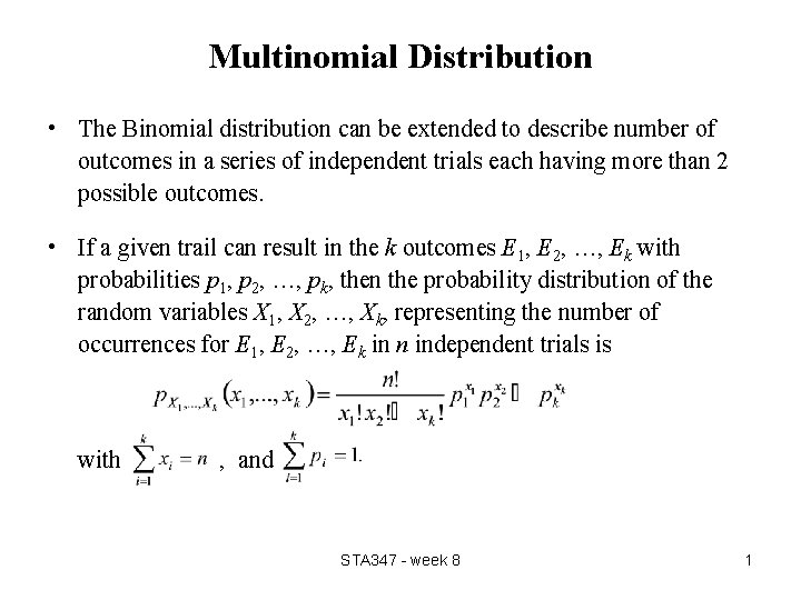
Multinomial Distribution • The Binomial distribution can be extended to describe number of outcomes in a series of independent trials each having more than 2 possible outcomes. • If a given trail can result in the k outcomes E 1, E 2, …, Ek with probabilities p 1, p 2, …, pk, then the probability distribution of the random variables X 1, X 2, …, Xk, representing the number of occurrences for E 1, E 2, …, Ek in n independent trials is with , and STA 347 - week 8 1

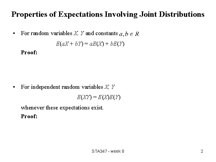
Properties of Expectations Involving Joint Distributions • For random variables X, Y and constants E(a. X + b. Y) = a. E(X) + b. E(Y) Proof: • For independent random variables X, Y E(XY) = E(X)E(Y) whenever these expectations exist. Proof: STA 347 - week 8 2

Covariance • Recall: Var(X+Y) = Var(X) + Var(Y) +2 E[(X-E(X))(Y-E(Y))] • Definition For random variables X, Y with E(X), E(Y) < ∞, the covariance of X and Y is • Covariance measures whether or not X-E(X) and Y-E(Y) have the same sign. • Claim: Proof: • Note: If X, Y independent then E(XY) =E(X)E(Y), and Cov(X, Y) = 0. STA 347 - week 8 3

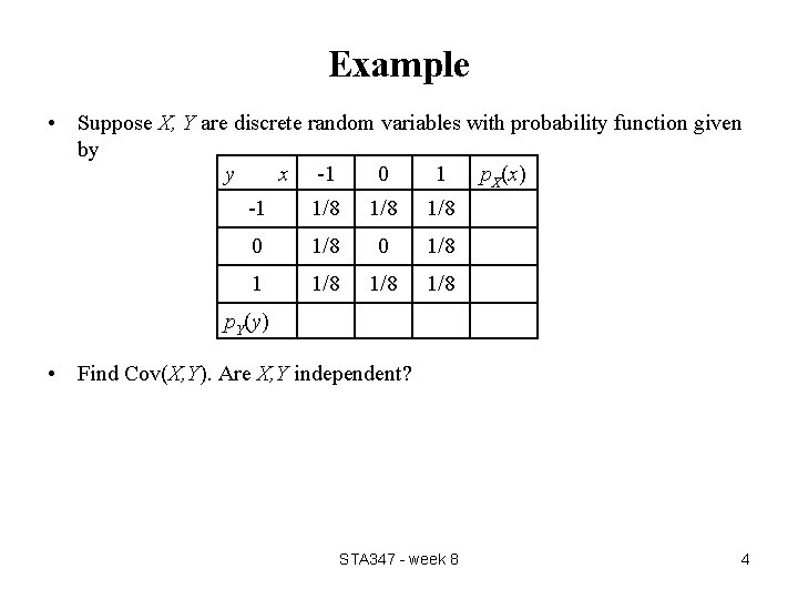
Example • Suppose X, Y are discrete random variables with probability function given by y x -1 0 1 p. X(x) -1 1/8 1/8 0 1/8 1/8 1/8 p. Y(y) • Find Cov(X, Y). Are X, Y independent? STA 347 - week 8 4

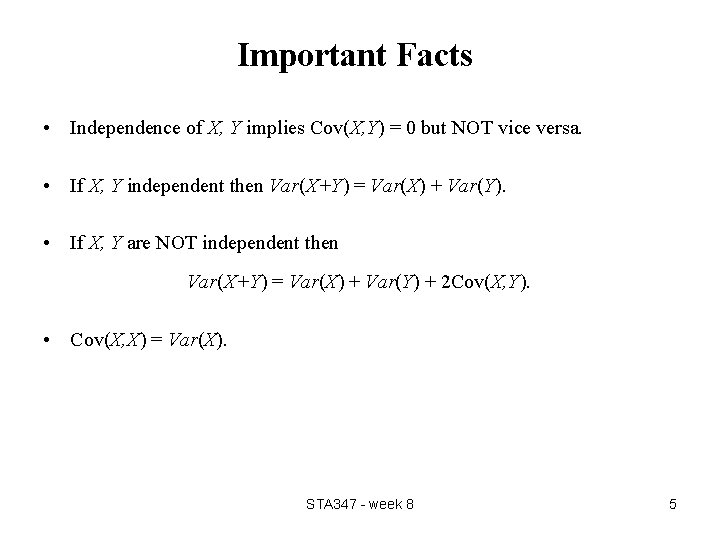
Important Facts • Independence of X, Y implies Cov(X, Y) = 0 but NOT vice versa. • If X, Y independent then Var(X+Y) = Var(X) + Var(Y). • If X, Y are NOT independent then Var(X+Y) = Var(X) + Var(Y) + 2 Cov(X, Y). • Cov(X, X) = Var(X). STA 347 - week 8 5

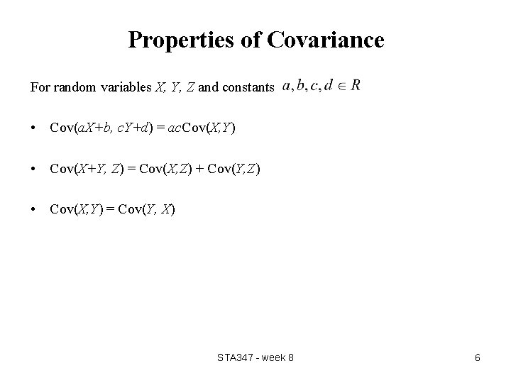
Properties of Covariance For random variables X, Y, Z and constants • Cov(a. X+b, c. Y+d) = ac. Cov(X, Y) • Cov(X+Y, Z) = Cov(X, Z) + Cov(Y, Z) • Cov(X, Y) = Cov(Y, X) STA 347 - week 8 6

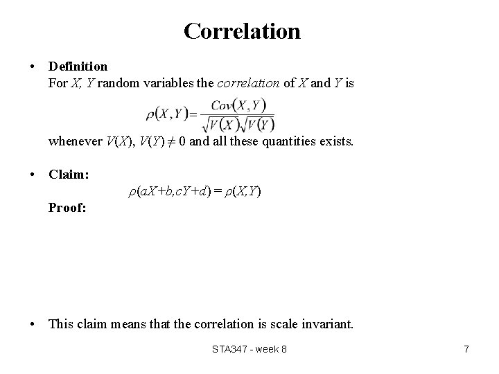
Correlation • Definition For X, Y random variables the correlation of X and Y is whenever V(X), V(Y) ≠ 0 and all these quantities exists. • Claim: ρ(a. X+b, c. Y+d) = ρ(X, Y) Proof: • This claim means that the correlation is scale invariant. STA 347 - week 8 7

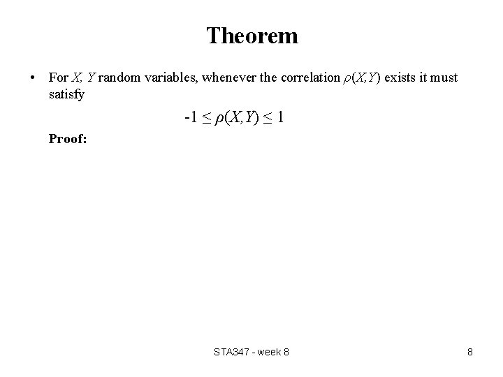
Theorem • For X, Y random variables, whenever the correlation ρ(X, Y) exists it must satisfy -1 ≤ ρ(X, Y) ≤ 1 Proof: STA 347 - week 8 8

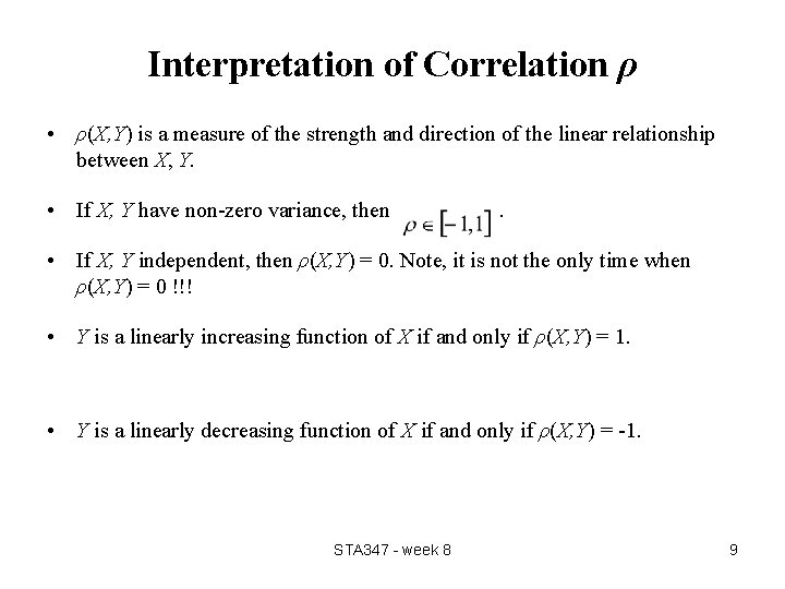
Interpretation of Correlation ρ • ρ(X, Y) is a measure of the strength and direction of the linear relationship between X, Y. • If X, Y have non-zero variance, then . • If X, Y independent, then ρ(X, Y) = 0. Note, it is not the only time when ρ(X, Y) = 0 !!! • Y is a linearly increasing function of X if and only if ρ(X, Y) = 1. • Y is a linearly decreasing function of X if and only if ρ(X, Y) = -1. STA 347 - week 8 9

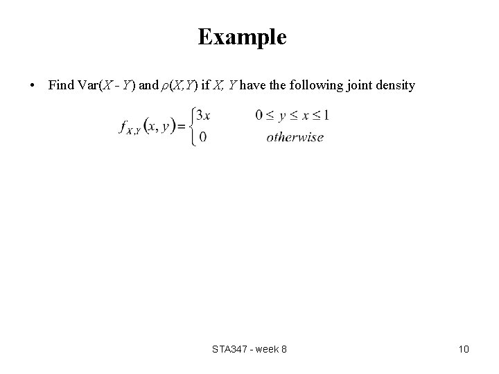
Example • Find Var(X - Y) and ρ(X, Y) if X, Y have the following joint density STA 347 - week 8 10

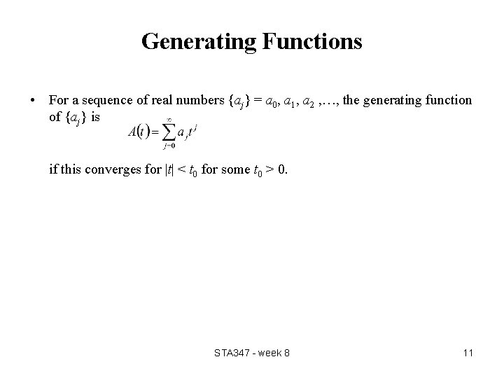
Generating Functions • For a sequence of real numbers {aj} = a 0, a 1, a 2 , …, the generating function of {aj} is if this converges for |t| < t 0 for some t 0 > 0. STA 347 - week 8 11

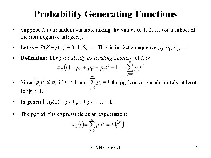
Probability Generating Functions • Suppose X is a random variable taking the values 0, 1, 2, … (or a subset of the non-negative integers). • Let pj = P(X = j) , j = 0, 1, 2, …. This is in fact a sequence p 0, p 1, p 2, … • Definition: The probability generating function of X is • Since for |t| < 1. if |t| < 1 and the pgf converges absolutely at least • In general, πX(1) = p 0 + p 1 + p 2 +… = 1. • The pgf of X is expressible as an expectation: STA 347 - week 8 12

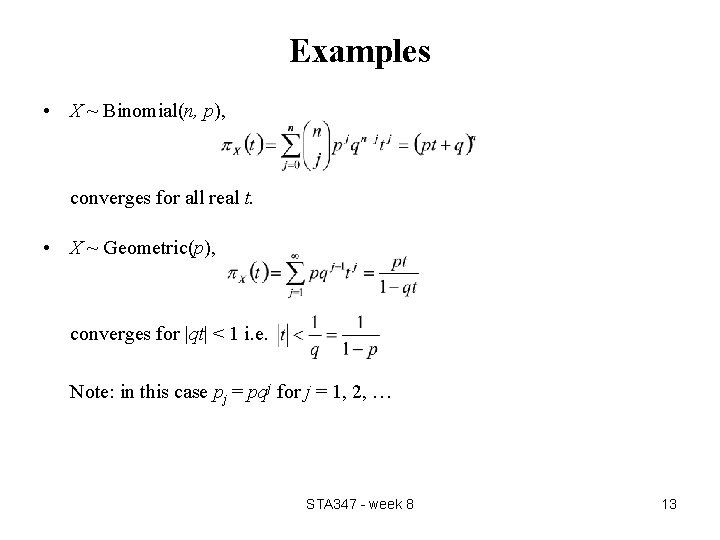
Examples • X ~ Binomial(n, p), converges for all real t. • X ~ Geometric(p), converges for |qt| < 1 i. e. Note: in this case pj = pqj for j = 1, 2, … STA 347 - week 8 13

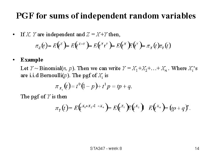
PGF for sums of independent random variables • If X, Y are independent and Z = X+Y then, • Example Let Y ~ Binomial(n, p). Then we can write Y = X 1+X 2+…+ Xn. Where Xi’s are i. i. d Bernoulli(p). The pgf of Xi is The pgf of Y is then STA 347 - week 8 14

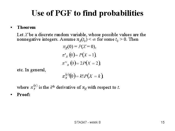
Use of PGF to find probabilities • Theorem Let X be a discrete random variable, whose possible values are the nonnegative integers. Assume πX(t 0) < ∞ for some t 0 > 0. Then πX(0) = P(X = 0), etc. In general, where • Proof: is the kth derivative of πX with respect to t. STA 347 - week 8 15

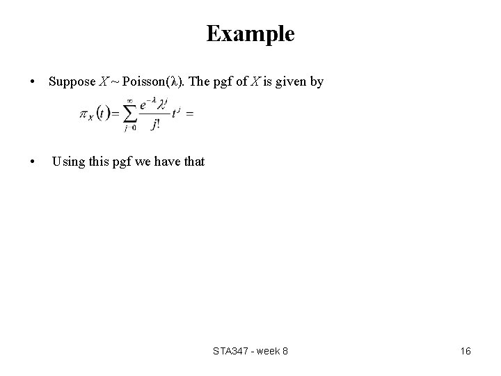
Example • Suppose X ~ Poisson(λ). The pgf of X is given by • Using this pgf we have that STA 347 - week 8 16

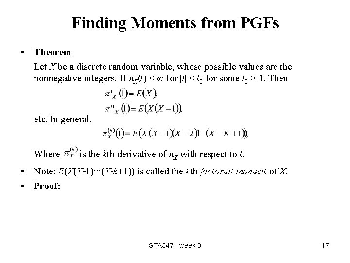
Finding Moments from PGFs • Theorem Let X be a discrete random variable, whose possible values are the nonnegative integers. If πX(t) < ∞ for |t| < t 0 for some t 0 > 1. Then etc. In general, Where is the kth derivative of πX with respect to t. • Note: E(X(X-1)∙∙∙(X-k+1)) is called the kth factorial moment of X. • Proof: STA 347 - week 8 17

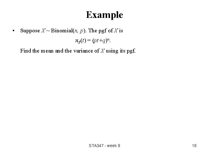
Example • Suppose X ~ Binomial(n, p). The pgf of X is πX(t) = (pt+q)n. Find the mean and the variance of X using its pgf. STA 347 - week 8 18

Uniqueness Theorem for PGF • Suppose X, Y have probability generating function πX and πY respectively. Then πX(t) = πY(t) if and only if P(X = k) = P(Y = k) for k = 0, 1, 2, … • Proof: Follow immediately from calculus theorem: If a function is expressible as a power series at x=a, then there is only one such series. A pgf is a power series about the origin which we know exists with radius of convergence of at least 1. STA 347 - week 8 19

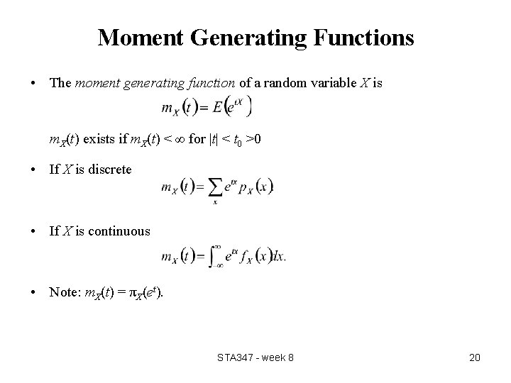
Moment Generating Functions • The moment generating function of a random variable X is m. X(t) exists if m. X(t) < ∞ for |t| < t 0 >0 • If X is discrete • If X is continuous • Note: m. X(t) = πX(et). STA 347 - week 8 20

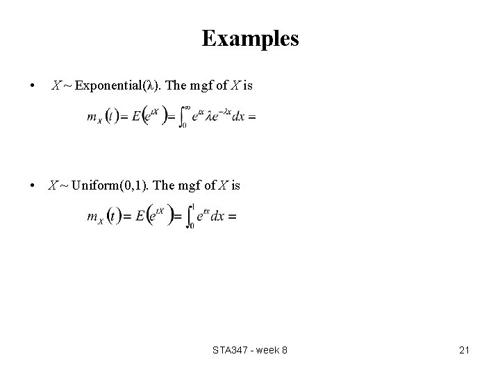
Examples • X ~ Exponential(λ). The mgf of X is • X ~ Uniform(0, 1). The mgf of X is STA 347 - week 8 21

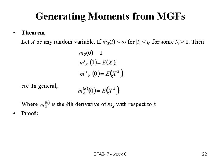
Generating Moments from MGFs • Theorem Let X be any random variable. If m. X(t) < ∞ for |t| < t 0 for some t 0 > 0. Then m. X(0) = 1 etc. In general, Where • Proof: is the kth derivative of m. X with respect to t. STA 347 - week 8 22

Example • Suppose X ~ Exponential(λ). Find the mean and variance of X using its moment generating function. STA 347 - week 8 23

Example • Suppose X ~ N(0, 1). Find the mean and variance of X using its moment generating function. STA 347 - week 8 24

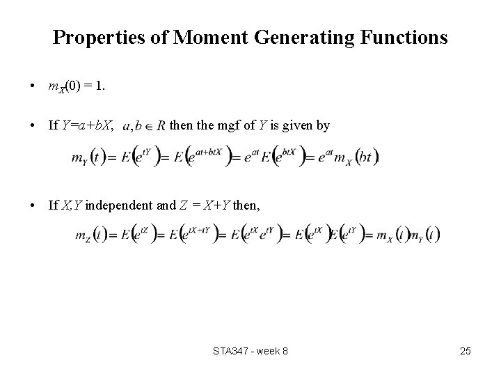
Properties of Moment Generating Functions • m. X(0) = 1. • If Y=a+b. X, then the mgf of Y is given by • If X, Y independent and Z = X+Y then, STA 347 - week 8 25

Uniqueness Theorem • If a moment generating function m. X(t) exists for t in an open interval containing 0, it uniquely determines the probability distribution. STA 347 - week 8 26

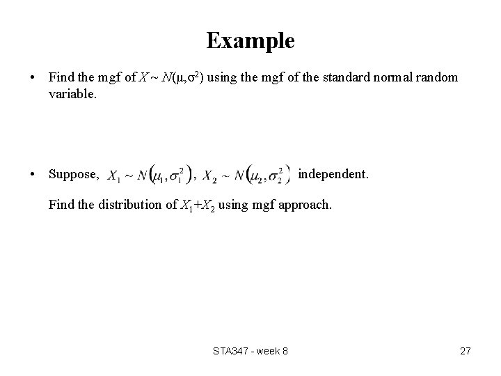
Example • Find the mgf of X ~ N(μ, σ2) using the mgf of the standard normal random variable. • Suppose, , independent. Find the distribution of X 1+X 2 using mgf approach. STA 347 - week 8 27

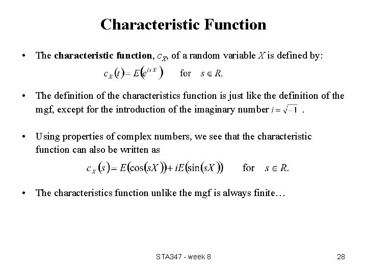
Characteristic Function • The characteristic function, c. X, of a random variable X is defined by: • The definition of the characteristics function is just like the definition of the mgf, except for the introduction of the imaginary number. • Using properties of complex numbers, we see that the characteristic function can also be written as • The characteristics function unlike the mgf is always finite… STA 347 - week 8 28

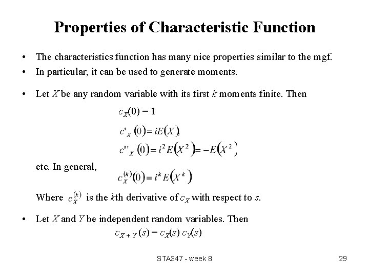
Properties of Characteristic Function • The characteristics function has many nice properties similar to the mgf. • In particular, it can be used to generate moments. • Let X be any random variable with its first k moments finite. Then c. X(0) = 1 etc. In general, Where is the kth derivative of c. X with respect to s. • Let X and Y be independent random variables. Then c. X + Y (s) = c. X(s) c. Y(s) STA 347 - week 8 29

Examples STA 347 - week 8 30