Multimedia Data Kien A Hua University of Central

Multimedia Data Kien A. Hua University of Central Florida Orlando FL 32816 -2362

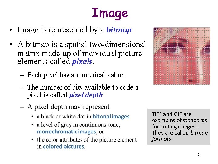
Image • Image is represented by a bitmap. • A bitmap is a spatial two-dimensional matrix made up of individual picture elements called pixels. – Each pixel has a numerical value. – The number of bits available to code a pixel is called pixel depth. TIFF and GIF are examples of standards for coding images. They are called bitmap formats. 2

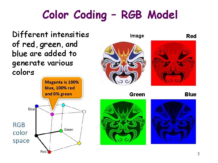
Color Coding – RGB Model Different intensities of red, green, and blue are added to generate various colors Magenta is 100% blue, 100% red and 0% green Image Red Green Blue RGB color space 3

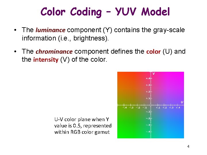
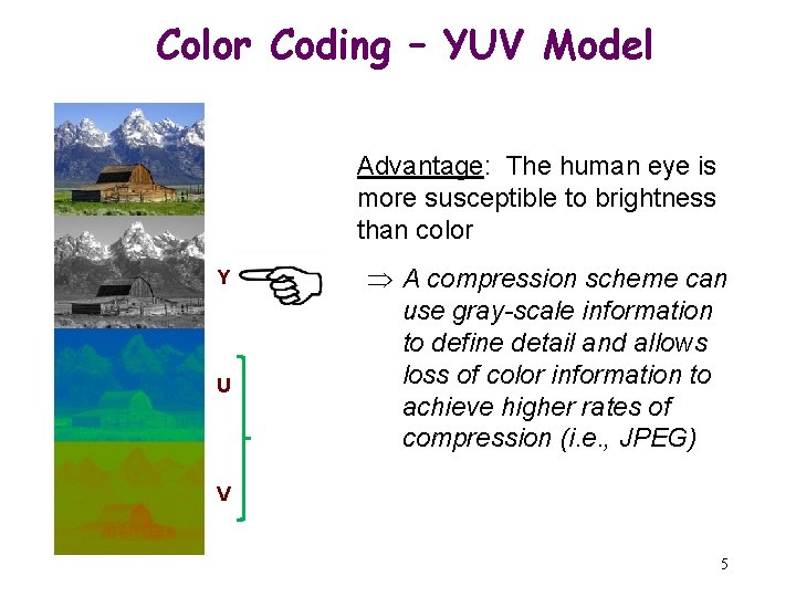
Color Coding – YUV Model • The luminance component (Y) contains the gray-scale information (i. e. , brightness). • The chrominance component defines the color (U) and the intensity (V) of the color. U-V color plane when Y value is 0. 5, represented within RGB color gamut 4

Color Coding – YUV Model Advantage: The human eye is more susceptible to brightness than color Y U A compression scheme can use gray-scale information to define detail and allows loss of color information to achieve higher rates of compression (i. e. , JPEG) V 5

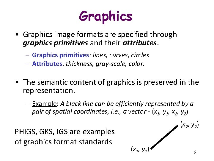
Graphics • Graphics image formats are specified through graphics primitives and their attributes. – Graphics primitives: lines, curves, circles – Attributes: thickness, gray-scale, color. • The semantic content of graphics is preserved in the representation. – Example: A black line can be efficiently represented by a pair of spatial coordinates, i. e. , a vector - (x 1, y 1, x 2, y 2). PHIGS, GKS, IGS are examples of graphics format standards (x 2, y 2) (x 1, y 1) 6

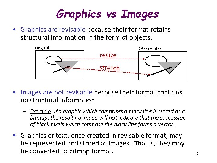
Graphics vs Images • Graphics are revisable because their format retains structural information in the form of objects. Original resize After revision stretch • Images are not revisable because their format contains no structural information. – Example: If a graphic which comprises a black line is stored as a bitmap, the resulting image will not indicate that the succession of black pixels which compose the black line forms a vector. • Graphics or text, once created in revisable format, may be represented and stored as images. That is, they may be converted to bitmap format. 7

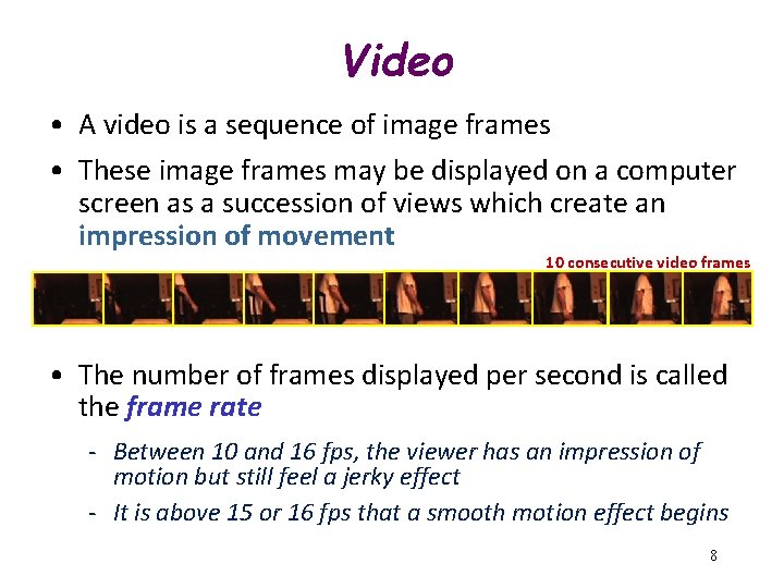
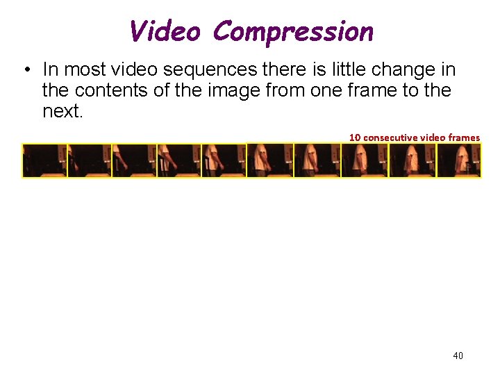
Video • A video is a sequence of image frames • These image frames may be displayed on a computer screen as a succession of views which create an impression of movement 10 consecutive video frames • The number of frames displayed per second is called the frame rate - Between 10 and 16 fps, the viewer has an impression of motion but still feel a jerky effect - It is above 15 or 16 fps that a smooth motion effect begins 8

Multimedia Objects Are Huge Data compression Reduces storage and bandwidth requirements 9

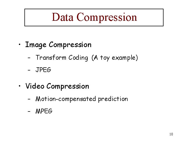
Data Compression • Image Compression – Transform Coding (A toy example) – JPEG • Video Compression – Motion-compensated prediction – MPEG 10

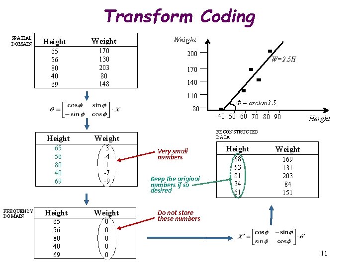
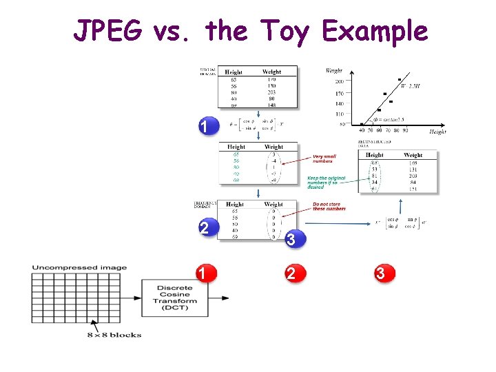
Transform Coding SPATIAL DOMAIN Height Weight 65 56 80 40 69 170 130 203 80 148 Weight 200 170 140 110 80 FREQUENCY DOMAIN Height Weight 65 56 80 40 69 3 -4 1 -7 -9 Height Weight 65 56 80 40 69 0 0 0 W=2. 5 H F = arctan 2. 5 40 50 60 70 80 90 Height RECONSTRUCTED DATA Very small numbers Keep the original numbers if so desired Height Weight 68 53 81 34 61 169 131 203 84 151 Do not store these numbers 11

Digital Signal Processing • A study of – signals in a digital representation, and – the processing methods of these signals. • A study of digital signals in – time domain (one-dimensional), – spatial domain (multidimensional), – frequency domain, etc. • Which domain to process a signal is an educated guess 12

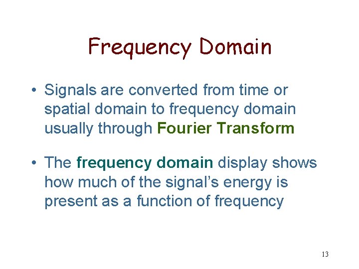
Frequency Domain • Signals are converted from time or spatial domain to frequency domain usually through Fourier Transform • The frequency domain display shows how much of the signal’s energy is present as a function of frequency 13

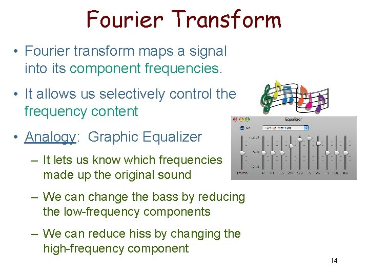
Fourier Transform • Fourier transform maps a signal into its component frequencies. • It allows us selectively control the frequency content • Analogy: Graphic Equalizer – It lets us know which frequencies made up the original sound – We can change the bass by reducing the low-frequency components – We can reduce hiss by changing the high-frequency component 14

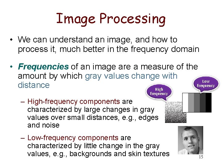
Image Processing • We can understand an image, and how to process it, much better in the frequency domain • Frequencies of an image are a measure of the amount by which gray values change with Low frequency distance High frequency – High-frequency components are characterized by large changes in gray values over small distances, e. g. , edges and noise – Low-frequency components are characterized by little change in the gray values, e. g. , backgrounds and skin textures 15

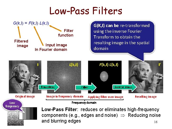
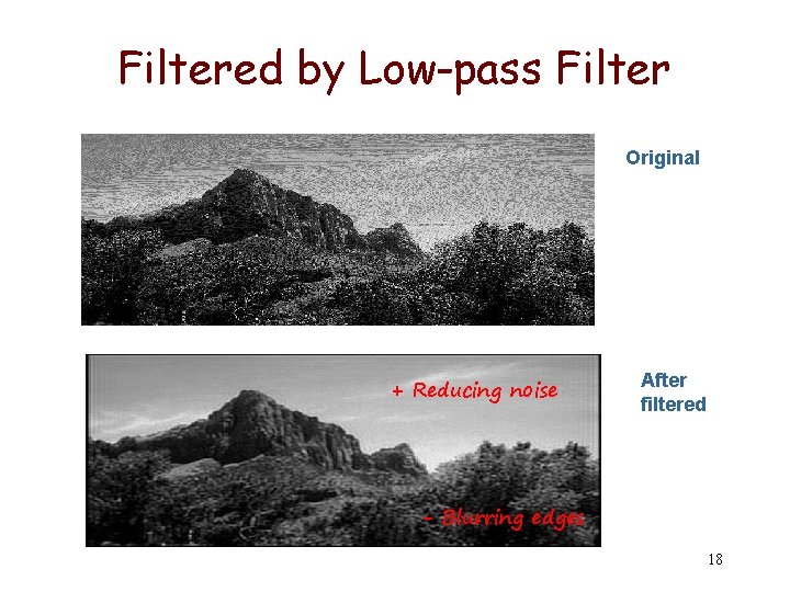
Low-Pass Filters G(k, l) = F(k, l) L(k, l) G(K, I) can be re-transformed using the inverse Fourier Transform to obtain the resulting image in the spatial domain Filter function Filtered image Input image In Fourier domain L(k, I) I Transform Original image Low frequency F(k, I) L(k, I) Filter Image in frequency domain I’ Inverse trans. Applying filter over image Resulting image Frequency domain Low-Pass Filter: reduces or eliminates high-frequency components (e. g. , edges and noise) Reducing noise and blurring edges 16

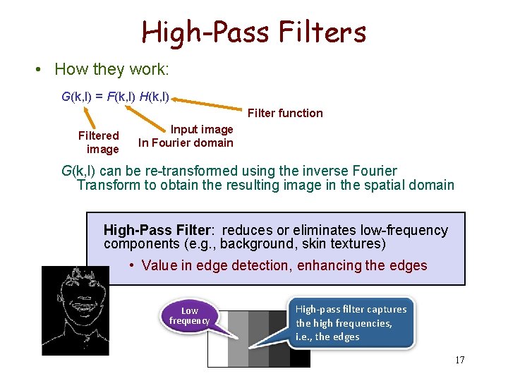
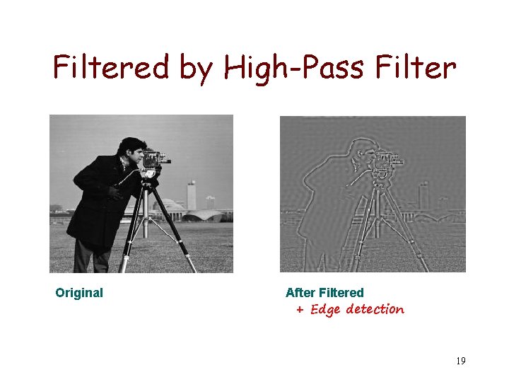
High-Pass Filters • How they work: G(k, l) = F(k, l) H(k, l) Filter function Filtered image Input image In Fourier domain G(k, l) can be re-transformed using the inverse Fourier Transform to obtain the resulting image in the spatial domain High-Pass Filter: reduces or eliminates low-frequency components (e. g. , background, skin textures) • Value in edge detection, enhancing the edges Low frequency High-pass filter captures the high frequencies, i. e. , the edges 17

Filtered by Low-pass Filter Original + Reducing noise After filtered - Blurring edges 18

Filtered by High-Pass Filter Original After Filtered + Edge detection 19

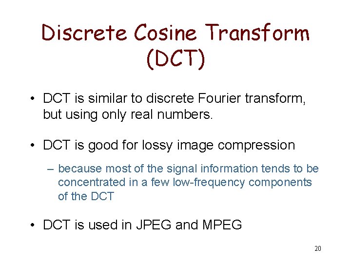
Discrete Cosine Transform (DCT) • DCT is similar to discrete Fourier transform, but using only real numbers. • DCT is good for lossy image compression – because most of the signal information tends to be concentrated in a few low-frequency components of the DCT • DCT is used in JPEG and MPEG 20

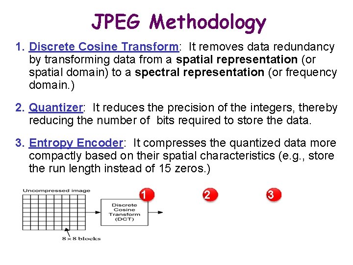
JPEG Methodology 1. Discrete Cosine Transform: It removes data redundancy by transforming data from a spatial representation (or spatial domain) to a spectral representation (or frequency domain. ) 2. Quantizer: It reduces the precision of the integers, thereby reducing the number of bits required to store the data. 3. Entropy Encoder: It compresses the quantized data more compactly based on their spatial characteristics (e. g. , store the run length instead of 15 zeros. ) 1 2 3 21

JPEG vs. the Toy Example 1 2 1 3 22

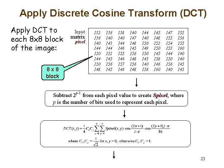
Apply Discrete Cosine Transform (DCT) Apply DCT to each 8 x 8 block of the image: 8 x 8 block Input matrix pixel 132 136 140 144 150 148 136 140 143 144 152 145 156 145 138 140 144 146 155 146 157 146 140 147 148 145 156 148 144 140 150 149 150 143 140 156 145 148 152 150 145 158 146 160 147 155 154 153 144 150 156 140 155 156 155 160 140 145 Subtract 2 p-1 from each pixel value to create Spixel, where p is the number of bits used to represent each pixel. 23

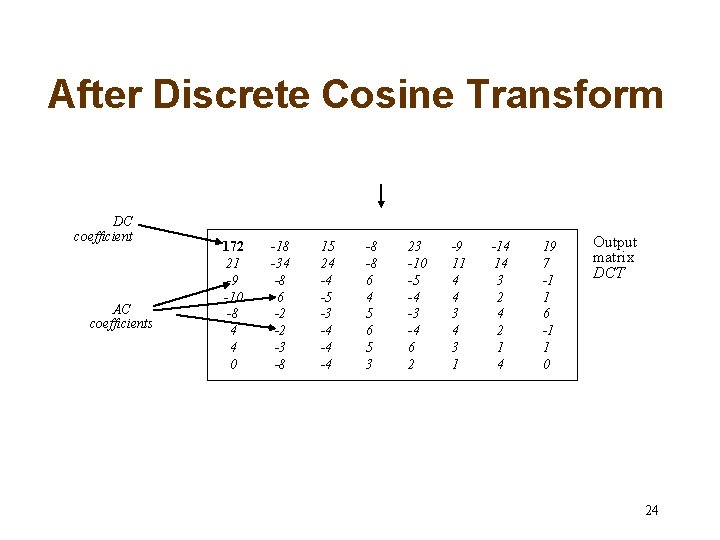
After Discrete Cosine Transform DC coefficient AC coefficients 172 21 -9 -10 -8 4 4 0 -18 -34 -8 6 -2 -2 -3 -8 15 24 -4 -5 -3 -4 -4 -4 -8 -8 6 4 5 6 5 3 23 -10 -5 -4 -3 -4 6 2 -9 11 4 4 3 1 -14 14 3 2 4 2 1 4 19 7 -1 1 6 -1 1 0 Output matrix DCT 24

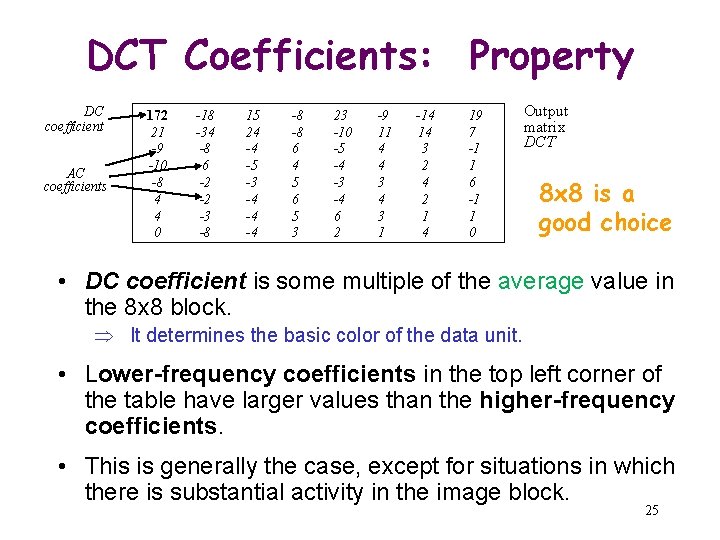
DCT Coefficients: Property DC coefficient AC coefficients 172 21 -9 -10 -8 4 4 0 -18 -34 -8 6 -2 -2 -3 -8 15 24 -4 -5 -3 -4 -4 -4 -8 -8 6 4 5 6 5 3 23 -10 -5 -4 -3 -4 6 2 -9 11 4 4 3 1 -14 14 3 2 4 2 1 4 19 7 -1 1 6 -1 1 0 Output matrix DCT 8 x 8 is a good choice • DC coefficient is some multiple of the average value in the 8 x 8 block. It determines the basic color of the data unit. • Lower-frequency coefficients in the top left corner of the table have larger values than the higher-frequency coefficients. • This is generally the case, except for situations in which there is substantial activity in the image block. 25

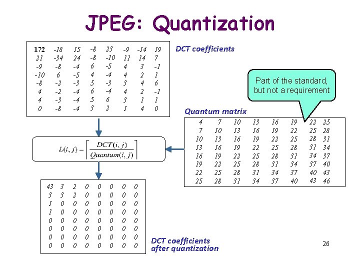
JPEG: Quantization 172 21 -9 -10 -8 4 4 0 -18 -34 -8 6 -2 -2 -3 -8 43 3 1 1 0 0 3 3 0 0 0 -8 -8 6 4 5 6 5 3 15 24 -4 -5 -3 -4 -4 -4 2 2 0 0 0 0 23 -10 -5 -4 -3 -4 6 2 0 0 0 0 -9 -14 11 14 4 3 4 2 3 4 4 2 3 1 1 4 0 0 0 0 19 7 -1 1 6 -1 1 0 DCT coefficients Part of the standard, but not a requirement Quantum matrix 4 7 10 13 16 19 22 25 28 DCT coefficients after quantization 10 13 16 19 22 25 28 31 34 37 40 22 25 28 31 34 37 40 43 46 26

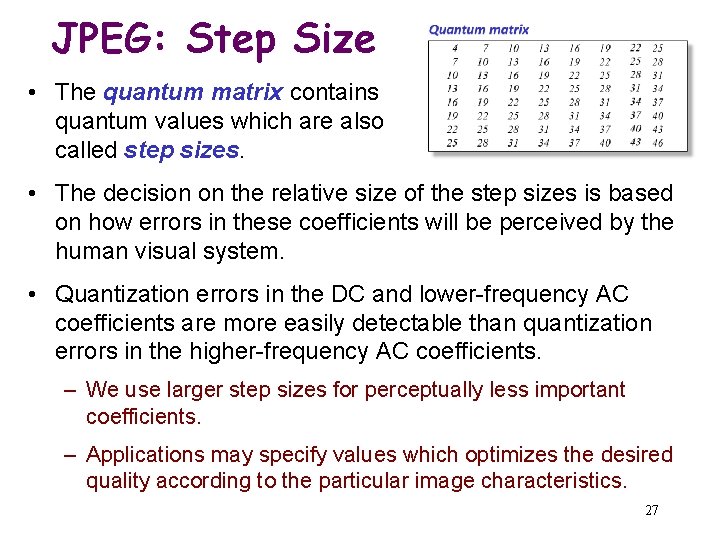
JPEG: Step Size • The quantum matrix contains quantum values which are also called step sizes. • The decision on the relative size of the step sizes is based on how errors in these coefficients will be perceived by the human visual system. • Quantization errors in the DC and lower-frequency AC coefficients are more easily detectable than quantization errors in the higher-frequency AC coefficients. – We use larger step sizes for perceptually less important coefficients. – Applications may specify values which optimizes the desired quality according to the particular image characteristics. 27

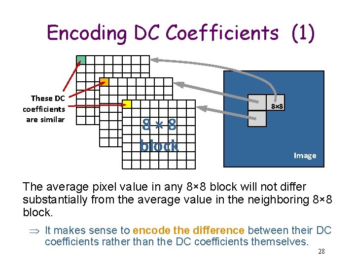
Encoding DC Coefficients (1) These DC coefficients are similar 8× 8 block Image The average pixel value in any 8× 8 block will not differ substantially from the average value in the neighboring 8× 8 block. It makes sense to encode the difference between their DC coefficients rather than the DC coefficients themselves. 28

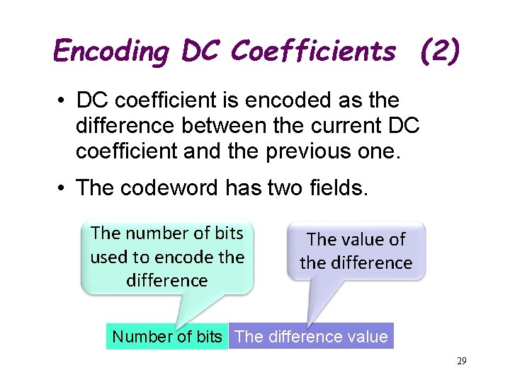
Encoding DC Coefficients (2) • DC coefficient is encoded as the difference between the current DC coefficient and the previous one. • The codeword has two fields. The number of bits used to encode the difference The value of the difference Number of bits The difference value 29

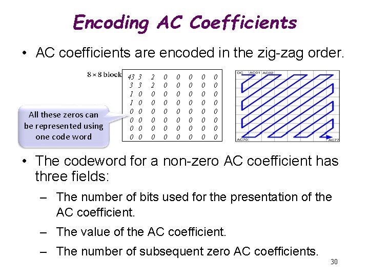
Encoding AC Coefficients • AC coefficients are encoded in the zig-zag order. All these zeros can be represented using one code word 43 3 1 1 0 0 3 3 0 0 0 2 2 0 0 0 0 0 0 0 0 0 0 0 0 • The codeword for a non-zero AC coefficient has three fields: – The number of bits used for the presentation of the AC coefficient. – The value of the AC coefficient. – The number of subsequent zero AC coefficients. 30

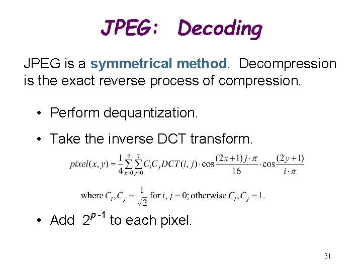
JPEG: Decoding JPEG is a symmetrical method. Decompression is the exact reverse process of compression. • Perform dequantization. • Take the inverse DCT transform. • Add 2 p -1 to each pixel. 31

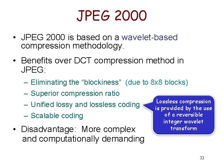
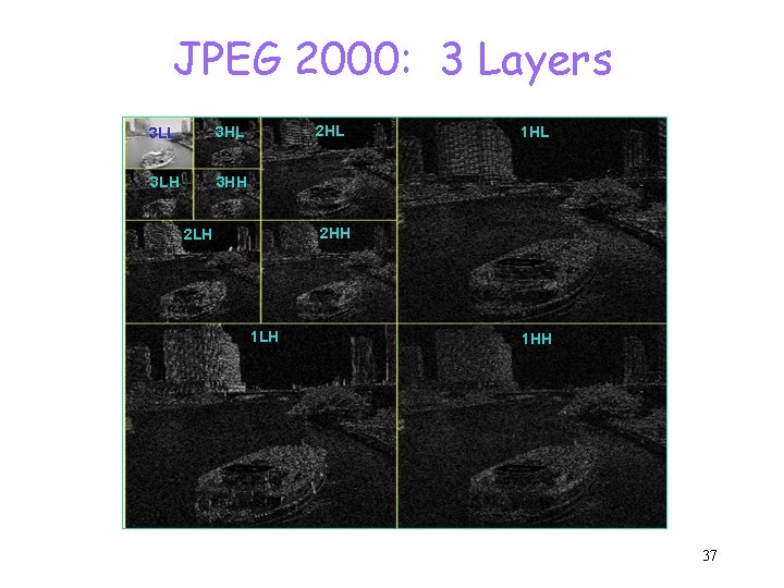
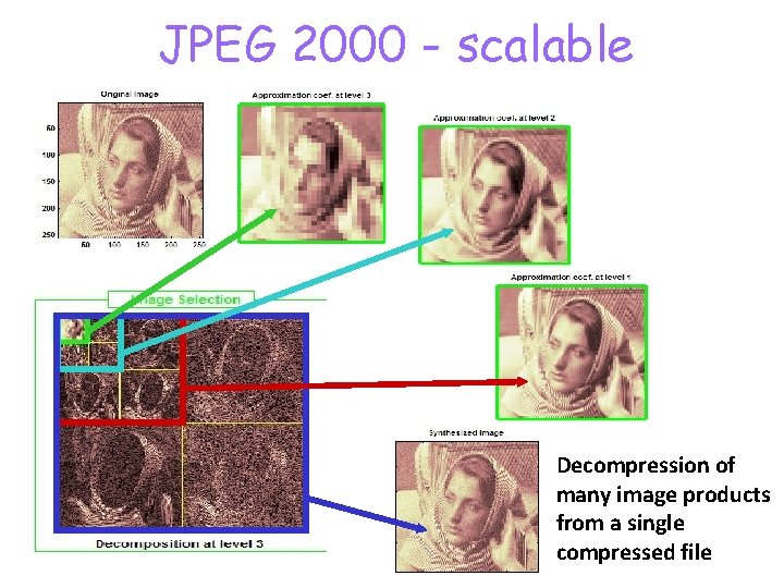
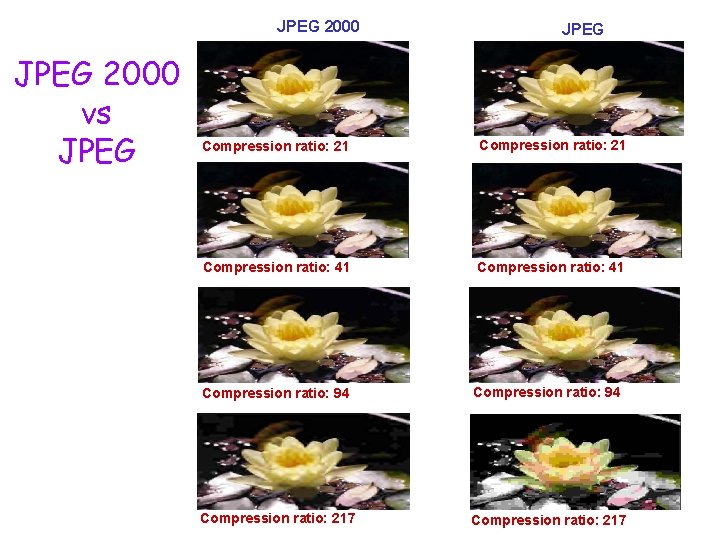
JPEG 2000 • JPEG 2000 is based on a wavelet-based compression methodology. • Benefits over DCT compression method in JPEG: – – Eliminating the “blockiness” (due to 8 x 8 blocks) Superior compression ratio Lossless compression Unified lossy and lossless coding is provided by the use of a reversible Scalable coding • Disadvantage: More complex and computationally demanding integer wavelet transform 32

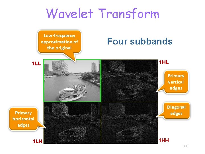
Wavelet Transform Low-frequency approximation of the original 1 LL Four subbands 1 HL Primary vertical edges Primary horizontal edges 1 LH Diagonal edges 1 HH 33

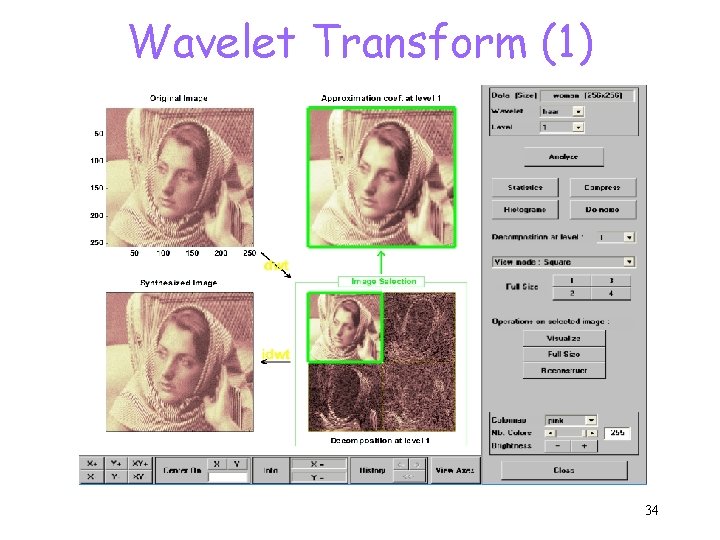
Wavelet Transform (1) 34

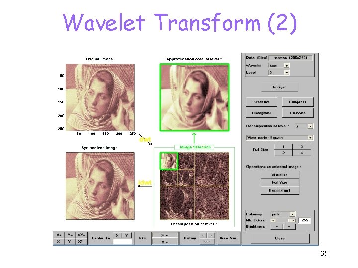
Wavelet Transform (2) 35

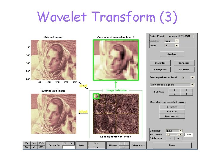
Wavelet Transform (3)

JPEG 2000: 3 Layers 3 LL 3 HL 3 LH 3 HH 2 HL 1 HL 2 HH 2 LH 1 HH 37

JPEG 2000 - scalable Decompression of many image products from a single compressed file

JPEG 2000 vs JPEG Compression ratio: 21 Compression ratio: 41 Compression ratio: 94 Compression ratio: 217

Video Compression • In most video sequences there is little change in the contents of the image from one frame to the next. 10 consecutive video frames 40

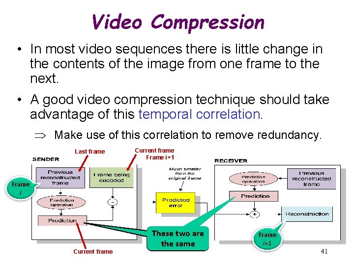
Video Compression • In most video sequences there is little change in the contents of the image from one frame to the next. • A good video compression technique should take advantage of this temporal correlation. Make use of this correlation to remove redundancy. Last frame Current frame Frame i+1 Frame i Current frame These two are the same Frame i+1 41

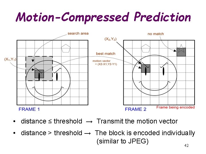
Motion-Compressed Prediction • distance ≤ threshold → Transmit the motion vector • distance > threshold → The block is encoded individually (similar to JPEG) 42

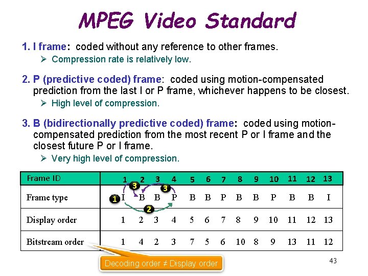
MPEG Video Standard 1. I frame: coded without any reference to other frames. Ø Compression rate is relatively low. 2. P (predictive coded) frame: coded using motion-compensated prediction from the last I or P frame, whichever happens to be closest. Ø High level of compression. 3. B (bidirectionally predictive coded) frame: coded using motioncompensated prediction from the most recent P or I frame and the closest future P or I frame. Ø Very high level of compression. Frame ID 4 5 6 7 8 9 10 11 12 13 P B B 3 4 5 6 7 8 9 10 11 12 13 2 3 7 5 6 10 8 9 13 11 12 2 3 1 I B B Display order 1 2 Bitstream order 1 4 Frame type 1 3 2 3 Decoding order ≠ Display order I 43

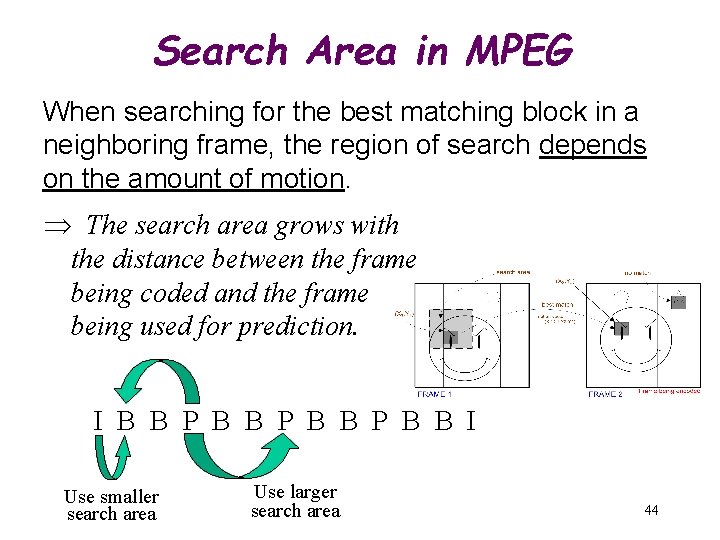
Search Area in MPEG When searching for the best matching block in a neighboring frame, the region of search depends on the amount of motion. The search area grows with the distance between the frame being coded and the frame being used for prediction. I B B P B B I Use smaller search area Use larger search area 44

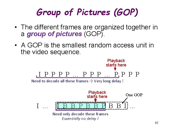
Group of Pictures (GOP) • The different frames are organized together in a group of pictures (GOP). • A GOP is the smallest random access unit in the video sequence. Playback starts here I P P … P P P P Need to decode all these frames → Very long delay ! Playback starts here I … One GOP I B B P B B I. . . Need only decode these frames Essentially no delay ! 45

Multimedia Operating Systems • Disk Scheduling • Admission Control • Deterministic Approach • Statistical Approach

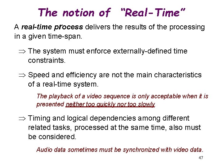
The notion of “Real-Time” A real-time process delivers the results of the processing in a given time-span. The system must enforce externally-defined time constraints. Speed and efficiency are not the main characteristics of a real-time system. The playback of a video sequence is only acceptable when it is presented neither too quickly nor too slowly. Timing and logical dependencies among different related tasks, processed at the same time, also must be considered. Audio data sometimes must be synchronized with video data. 47

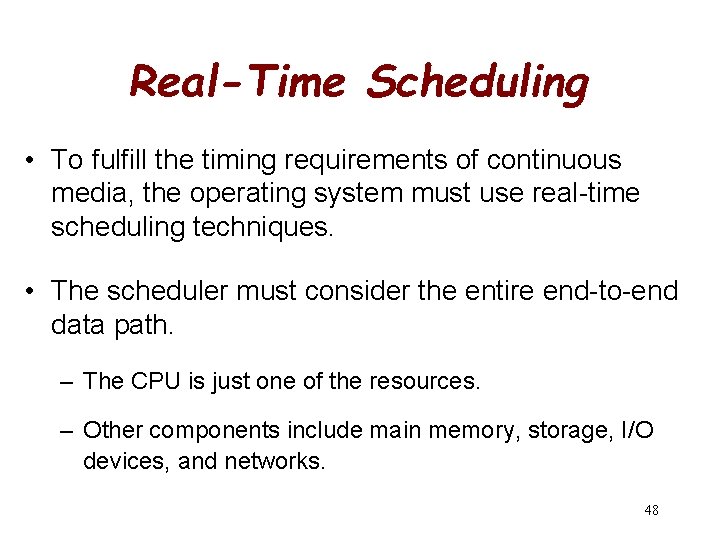
Real-Time Scheduling • To fulfill the timing requirements of continuous media, the operating system must use real-time scheduling techniques. • The scheduler must consider the entire end-to-end data path. – The CPU is just one of the resources. – Other components include main memory, storage, I/O devices, and networks. 48

Multimedia File Systems Conventional file systems: • Provide no rate guarantees for data retrieval. • Unsuitable for continuous media data (e. g. , 30 frames per second). Continuous media file systems: • Guarantee that once a request is accepted, data are retrieved at the requested rate. 49

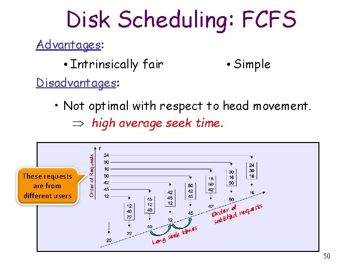
Disk Scheduling: FCFS Advantages: • Intrinsically fair Disadvantages: • Simple • Not optimal with respect to head movement. high average seek time. These requests are from different users g Lon tim seek es of quests r e Ord fied re s sati 50

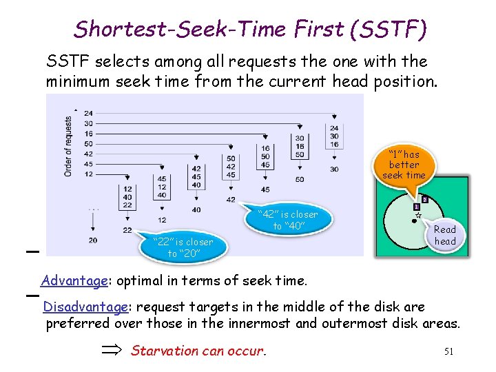
Shortest-Seek-Time First (SSTF) SSTF selects among all requests the one with the minimum seek time from the current head position. “ 1” has better seek time 2 “ 42” is closer to “ 40” “ 22” is closer to “ 20” 1 Read head Advantage: optimal in terms of seek time. Disadvantage: request targets in the middle of the disk are preferred over those in the innermost and outermost disk areas. Starvation can occur. 51

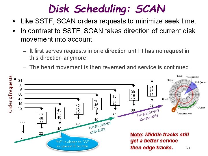
Disk Scheduling: SCAN • Like SSTF, SCAN orders requests to minimize seek time. • In contrast to SSTF, SCAN takes direction of current disk movement into account. – It first serves requests in one direction until it has no request in this direction anymore. Order of requests – The head movement is then reversed and service is continued. 24 30 16 50 42 45 12 . . . 12 40 22 45 12 40 22 20 42 45 12 oves m d a He rds upwa “ 40” is closer to “ 22” in upward direction 24 30 50 45 42 40 50 45 12 16 50 12 30 16 12 24 16 12 oves m d s Hea ward n w o d Note: Middle tracks still get a better service 52 then edge tracks.

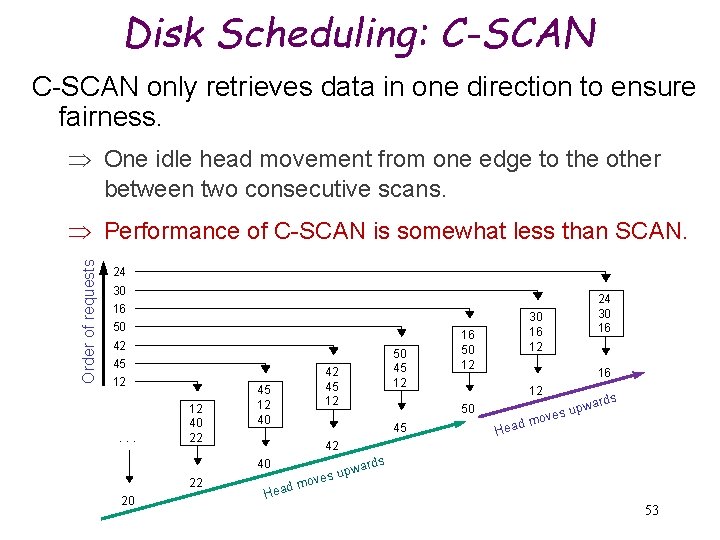
Disk Scheduling: C-SCAN only retrieves data in one direction to ensure fairness. One idle head movement from one edge to the other between two consecutive scans. Order of requests Performance of C-SCAN is somewhat less than SCAN. 24 30 16 50 42 45 12 . . . 12 40 22 42 45 12 40 20 16 50 12 16 12 50 45 d Hea ards pw es u v o m 42 40 22 50 45 12 30 16 12 24 30 16 v d mo Hea s ward p u es 53

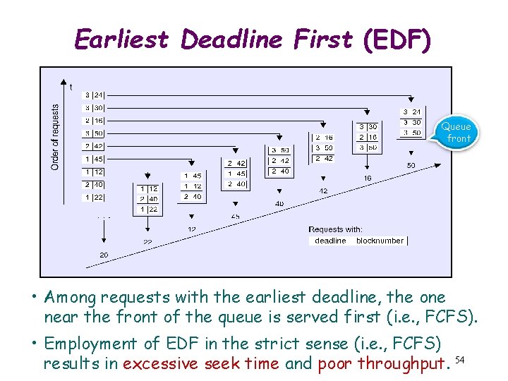
Earliest Deadline First (EDF) Queue front • Among requests with the earliest deadline, the one near the front of the queue is served first (i. e. , FCFS). • Employment of EDF in the strict sense (i. e. , FCFS) results in excessive seek time and poor throughput. 54

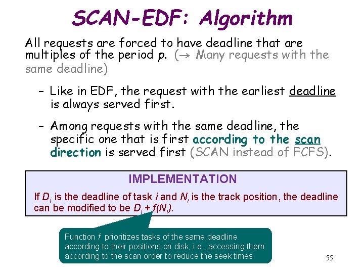
SCAN-EDF: Algorithm All requests are forced to have deadline that are multiples of the period p. (→ Many requests with the same deadline) – Like in EDF, the request with the earliest deadline is always served first. – Among requests with the same deadline, the specific one that is first according to the scan direction is served first (SCAN instead of FCFS). IMPLEMENTATION If Di is the deadline of task i and Ni is the track position, the deadline can be modified to be Di + f(Ni). Function f prioritizes tasks of the same deadline according to their positions on disk, i. e. , accessing them according to the scan order to reduce the seek times 55

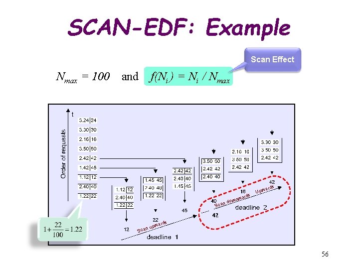
SCAN-EDF: Example Scan Effect Nmax = 100 and f(Ni ) = Ni / Nmax ward wn n do s Upw ards Sca 42 nu Sca rds pwa 56

SCAN-EDF: Advantages • EDF: Not optimal with respect to disk movement. • SCAN: Not taking deadline into account. • SCAN-EDF: Having the benefits of both EDF and SCAN. 57

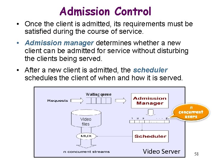
Admission Control • Once the client is admitted, its requirements must be satisfied during the course of service. • Admission manager determines whether a new client can be admitted for service without disturbing the clients being served. • After a new client is admitted, the scheduler schedules the client of when and how it is served. Waiting queue Video files n concurrent users Video Server 58

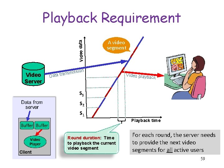
Video data Playback Requirement Video Server A video segment ssion ansmi Data tr Video playba ck S 3 S 2 S 1 Playback time Round duration: Time to playback the current video segment For each round, the server needs to provide the next video segments for all active users 59

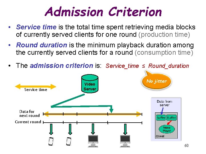
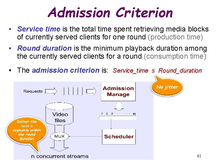
Admission Criterion • Service time is the total time spent retrieving media blocks of currently served clients for one round (production time) • Round duration is the minimum playback duration among the currently served clients for a round (consumption time) • The admission criterion is: Service_time ≤ Round_duration Service time Video Server No jitter Data for next round Current round 60

Admission Criterion • Service time is the total time spent retrieving media blocks of currently served clients for one round (production time) • Round duration is the minimum playback duration among the currently served clients for a round (consumption time) • The admission criterion is: Service_time ≤ Round_duration No jitter Deliver the next n segments within the round duration 61

Admission Control: Goals • High Throughput - Serve as many clients as possible per time unit. • High Utilization - Maximize resource utilization. • Minimum Latency - Offer minimum service delay for clients. 62

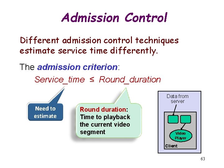
Admission Control Different admission control techniques estimate service time differently. The admission criterion: Service_time ≤ Round_duration Data from server Need to estimate Round duration: Time to playback the current video segment Video Player Client 63

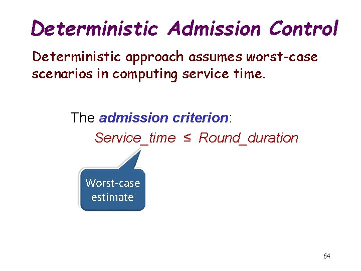
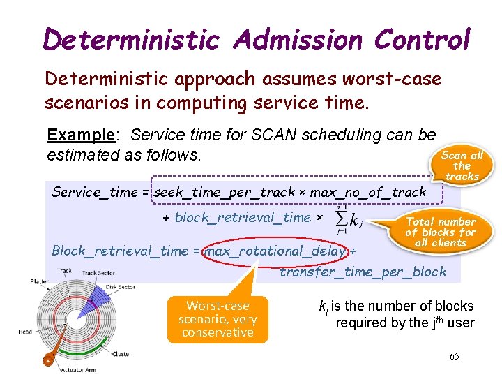
Deterministic Admission Control Deterministic approach assumes worst-case scenarios in computing service time. The admission criterion: Service_time ≤ Round_duration Worst-case estimate 64

Deterministic Admission Control Deterministic approach assumes worst-case scenarios in computing service time. Example: Service time for SCAN scheduling can be Scan all estimated as follows. Service_time = seek_time_per_track × max_no_of_track + block_retrieval_time × Block_retrieval_time = max_rotational_delay + the tracks Total number of blocks for all clients transfer_time_per_block Worst-case scenario, very conservative kj is the number of blocks required by the jth user 65

Deterministic Admission Control: Advantages • Advantages: - Continuity requirements of each client are not violated during the entire course of their playback. - The admission control algorithm is easy to implement. • Disadvantages: - The media server is underutilized since the average time for retrieving a block is usually much lower than the worst case value. - The throughput of the system is much less than the peak one. 66

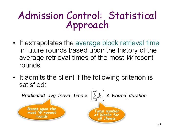
Admission Control: Statistical Approach • It extrapolates the average block retrieval time in future rounds based upon the history of the average retrieval times of the most W recent rounds. • It admits the client if the following criterion is satisfied: Predicated_avg_trieval_time × Based upon the most W recent rounds ≤ Round_duration Total number of blocks for all clients 67

Statistical Approach Advantage: – Server resources are better utilized – throughput is significantly increased Disadvantages: – It does not provide absolute guarantee to the clients since the algorithm employs prediction There are overflow rounds (some clients do not get the data) Several techniques can be applied to distribute the media loss among clients 68 – The algorithm is more complicated to implement.

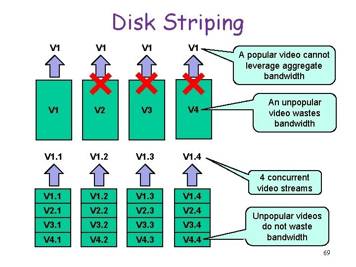
Disk Striping V 1 V 1 V 1 V 2 V 3 V 4 V 1. 1 V 1. 2 V 1. 3 V 1. 4 V 2. 1 V 2. 2 V 2. 3 V 2. 4 V 3. 1 V 3. 2 V 3. 3 V 3. 4 V 4. 1 V 4. 2 V 4. 3 V 4. 4 A popular video cannot leverage aggregate bandwidth An unpopular video wastes bandwidth 4 concurrent video streams Unpopular videos do not waste bandwidth 69

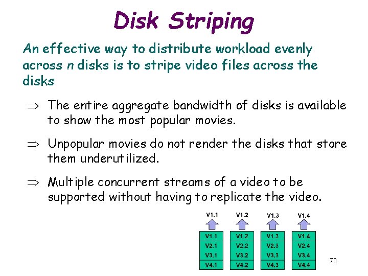
Disk Striping An effective way to distribute workload evenly across n disks is to stripe video files across the disks The entire aggregate bandwidth of disks is available to show the most popular movies. Unpopular movies do not render the disks that store them underutilized. Multiple concurrent streams of a video to be supported without having to replicate the video. 70