Multilevel Logic Synthesis Giovanni De Micheli Integrated Systems

Multi-level Logic Synthesis Giovanni De Micheli Integrated Systems Laboratory This presentation can be used for non-commercial purposes as long as this note and the copyright footers are not removed © Giovanni De Micheli – All rights reserved

Module 1 u Objectives s What is multi-level logic synthesis s What are the specific goals s Stepwise transformations (c) Giovanni De Micheli 2

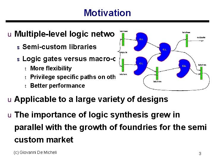
Motivation u Multiple-level logic networks s Semi-custom libraries s Logic gates versus macro-cells t t t More flexibility Privilege specific paths on others Better performance u Applicable to a large variety of designs u The importance of logic synthesis grew in parallel with the growth of foundries for the semi custom market (c) Giovanni De Micheli 3

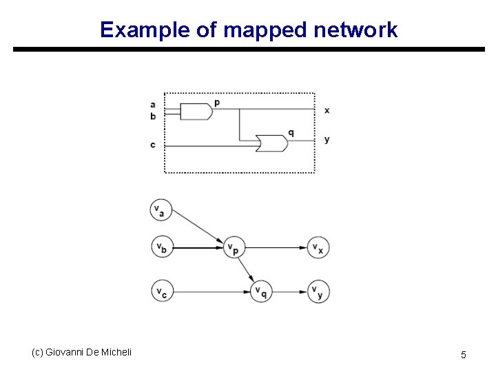
Circuit model u Logic network s An interconnection of blocks t s Each block modeled by a Boolean function Usual restrictions: t t Acyclic and memoryless Single-output functions u The model has a structural/behavioral semantics s The structure is induced by the interconnection u Mapped network Special case when the blocks correspond to library elements (c) Giovanni De Micheli s 4

Example of mapped network (c) Giovanni De Micheli 5

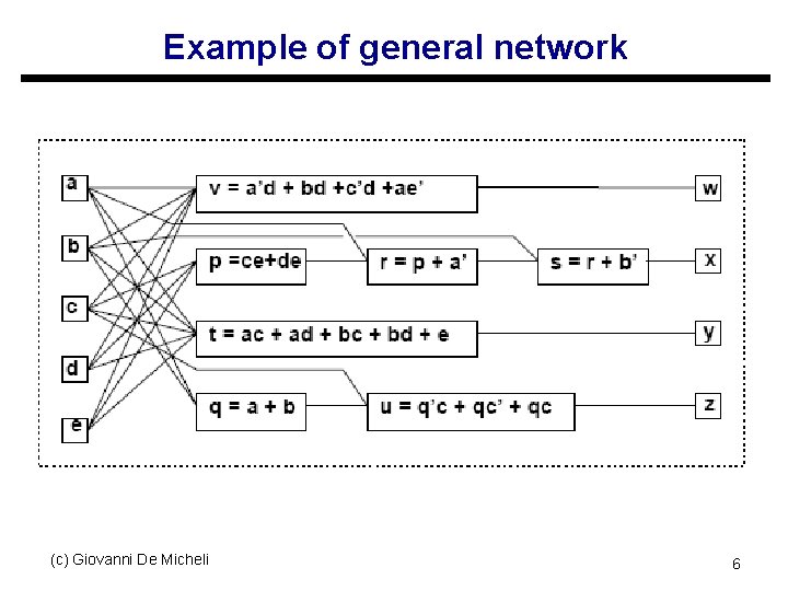
Example of general network (c) Giovanni De Micheli 6

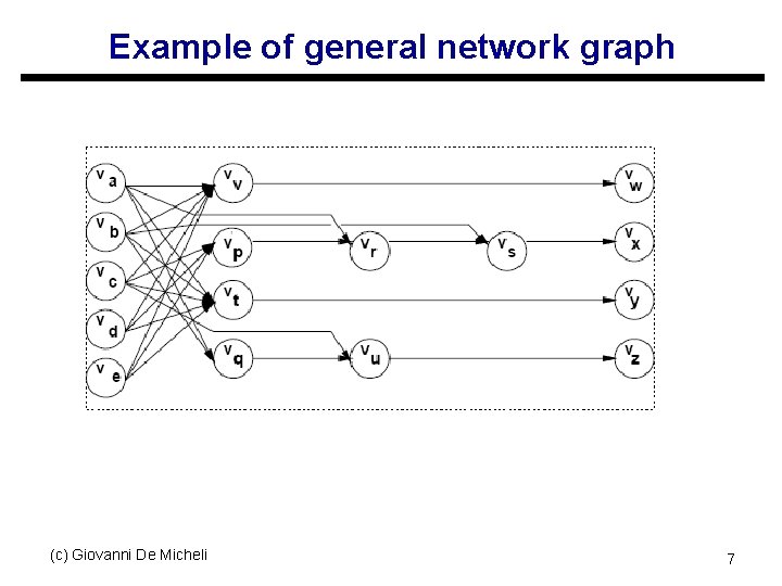
Example of general network graph (c) Giovanni De Micheli 7

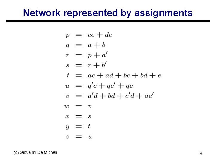
Network represented by assignments (c) Giovanni De Micheli 8

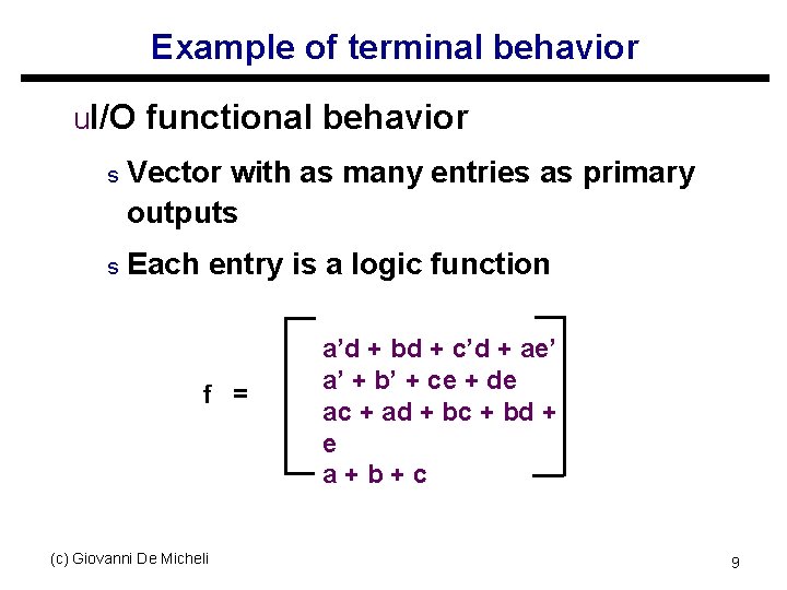
Example of terminal behavior u. I/O functional behavior s Vector with as many entries as primary outputs s Each entry is a logic function f = (c) Giovanni De Micheli a’d + bd + c’d + ae’ a’ + b’ + ce + de ac + ad + bc + bd + e a+b+c 9

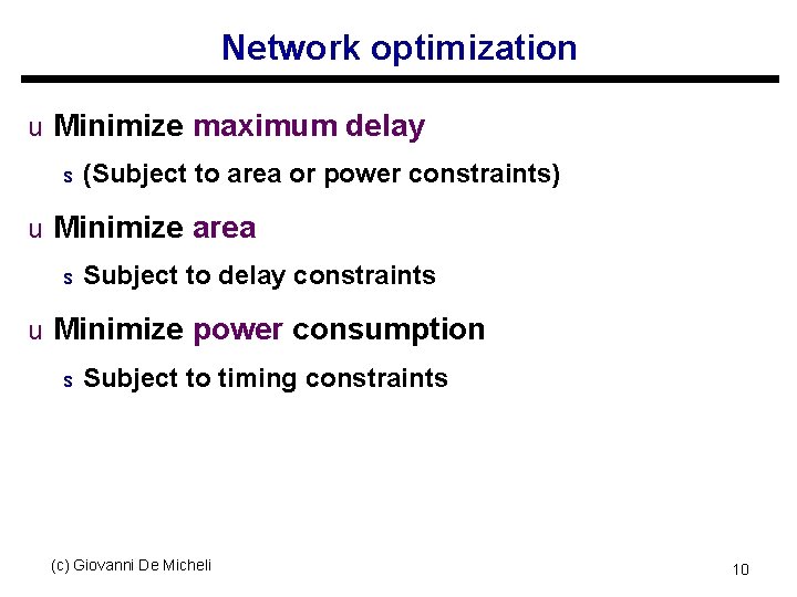
Network optimization u Minimize maximum delay s (Subject to area or power constraints) u Minimize area s Subject to delay constraints u Minimize power consumption s Subject to timing constraints (c) Giovanni De Micheli 10

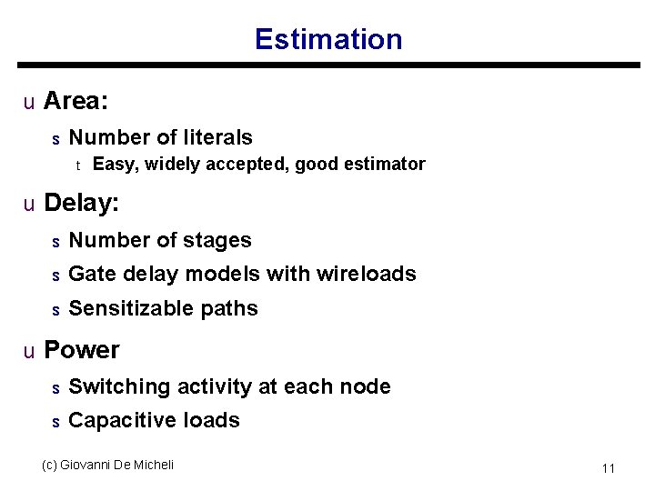
Estimation u Area: s Number of literals t Easy, widely accepted, good estimator u Delay: s Number of stages s Gate delay models with wireloads s Sensitizable paths u Power s Switching activity at each node s Capacitive loads (c) Giovanni De Micheli 11

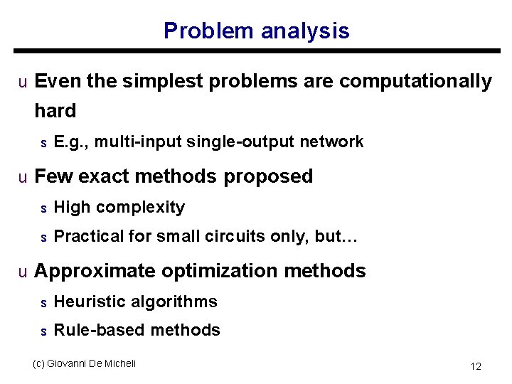
Problem analysis u Even the simplest problems are computationally hard s E. g. , multi-input single-output network u Few exact methods proposed s High complexity s Practical for small circuits only, but… u Approximate optimization methods s Heuristic algorithms s Rule-based methods (c) Giovanni De Micheli 12

Strategies for optimization u Improve network step by step s Circuit transformations u Preserve network I/O behavior s Exploit environment don’t cares if desired u Methods differ in: s Types of transformations applied s Selection and order of the transformations (c) Giovanni De Micheli 13

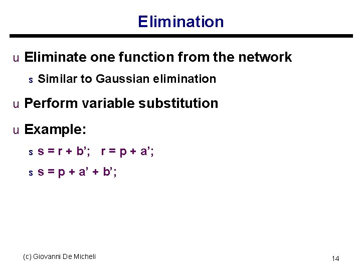
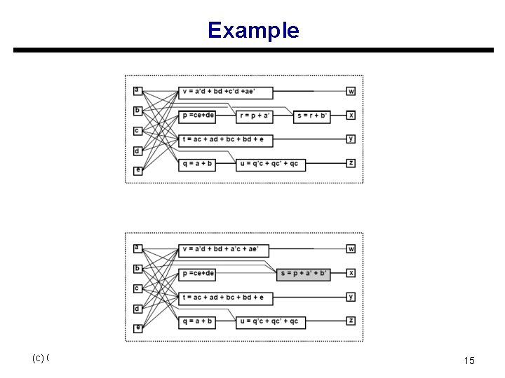
Elimination u Eliminate one function from the network s Similar to Gaussian elimination u Perform variable substitution u Example: s s = r + b’; r = p + a’; s s = p + a’ + b’; (c) Giovanni De Micheli 14

Example (c) Giovanni De Micheli 15

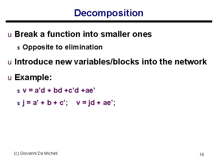
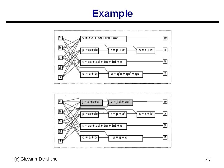
Decomposition u Break a function into smaller ones s Opposite to elimination u Introduce new variables/blocks into the network u Example: s v = a’d + bd +c’d +ae’ s j = a’ + b + c’; (c) Giovanni De Micheli v = jd + ae’; 16

Example (c) Giovanni De Micheli 17

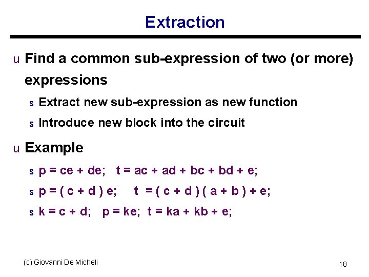
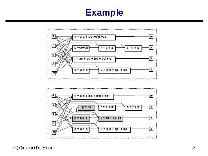
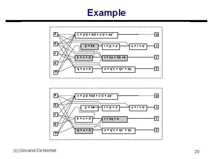
Extraction u Find a common sub-expression of two (or more) expressions s Extract new sub-expression as new function s Introduce new block into the circuit u Example s p = ce + de; t = ac + ad + bc + bd + e; s p = ( c + d ) e; s k = c + d; p = ke; t = ka + kb + e; (c) Giovanni De Micheli t = ( c + d ) ( a + b ) + e; 18

Example (c) Giovanni De Micheli 19

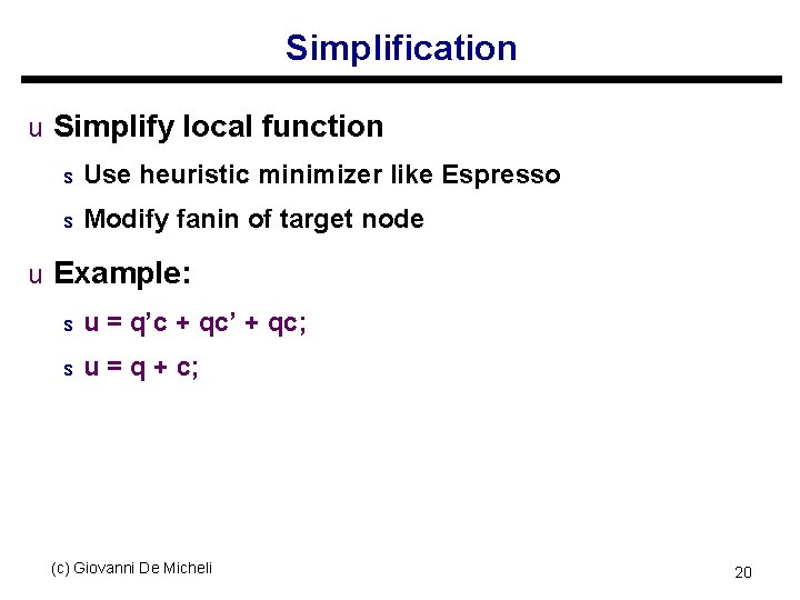
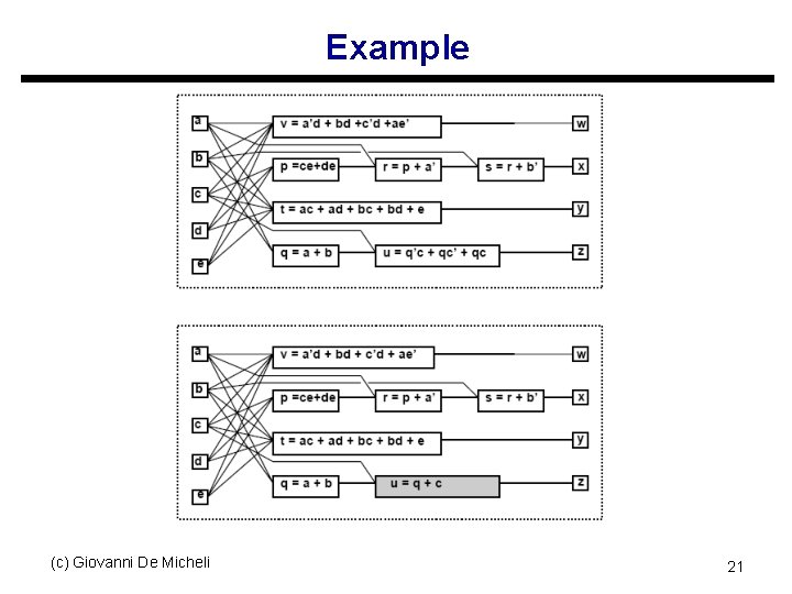
Simplification u Simplify local function s Use heuristic minimizer like Espresso s Modify fanin of target node u Example: s u = q’c + qc’ + qc; s u = q + c; (c) Giovanni De Micheli 20

Example (c) Giovanni De Micheli 21

Substitution u Simplify a local function by using an additional input that was not previously in its support set u Example: s t = ka + kb + e; s t = kq + e; s Because q = a + b is already part of the network (c) Giovanni De Micheli 22

Example (c) Giovanni De Micheli 23

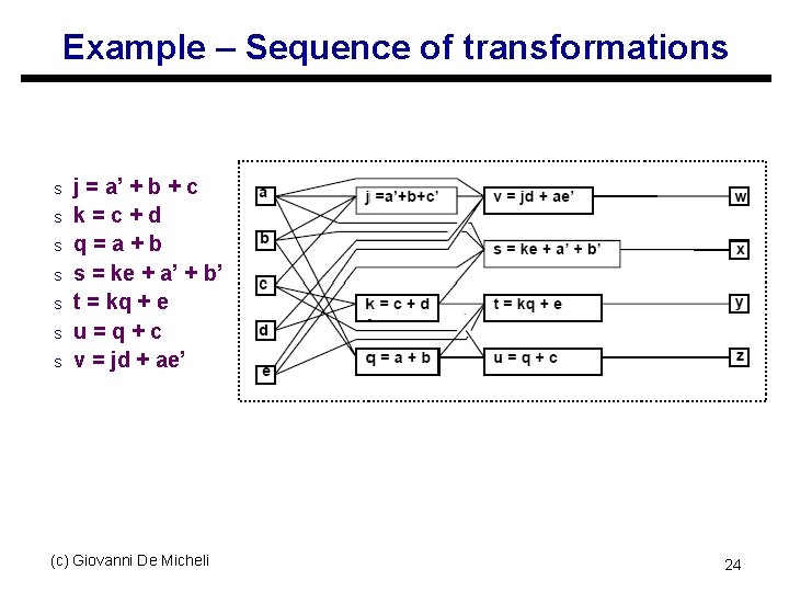
Example – Sequence of transformations s s s j = a’ + b + c k=c+d q=a+b s = ke + a’ + b’ t = kq + e u=q+c v = jd + ae’ (c) Giovanni De Micheli 24

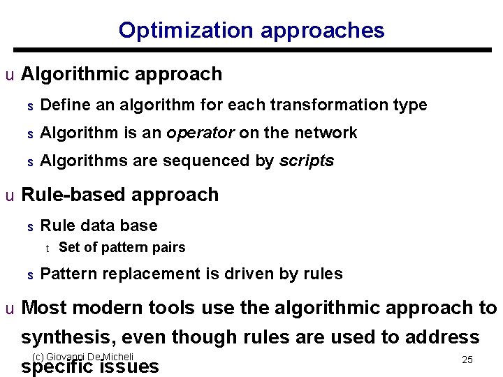
Optimization approaches u Algorithmic approach s Define an algorithm for each transformation type s Algorithm is an operator on the network s Algorithms are sequenced by scripts u Rule-based approach s Rule data base t s Set of pattern pairs Pattern replacement is driven by rules u Most modern tools use the algorithmic approach to synthesis, even though rules are used to address (c) Giovanni De Micheli specific issues 25

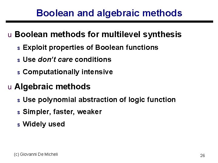
Boolean and algebraic methods u Boolean methods for multilevel synthesis s Exploit properties of Boolean functions s Use don’t care conditions s Computationally intensive u Algebraic methods s Use polynomial abstraction of logic function s Simpler, faster, weaker s Widely used (c) Giovanni De Micheli 26

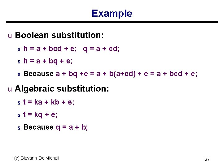
Example u Boolean substitution: s h = a + bcd + e; q = a + cd; s h = a + bq + e; s Because a + bq +e = a + b(a+cd) + e = a + bcd + e; u Algebraic substitution: s t = ka + kb + e; s t = kq + e; s Because q = a + b; (c) Giovanni De Micheli 27

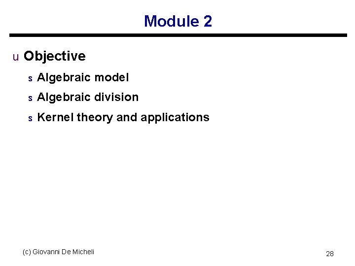
Module 2 u Objective s Algebraic model s Algebraic division s Kernel theory and applications (c) Giovanni De Micheli 28

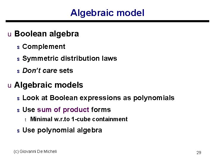
Algebraic model u Boolean algebra s Complement s Symmetric distribution laws s Don’t care sets u Algebraic models s Look at Boolean expressions as polynomials s Use sum of product forms t s Minimal w. r. to 1 -cube containment Use polynomial algebra (c) Giovanni De Micheli 29

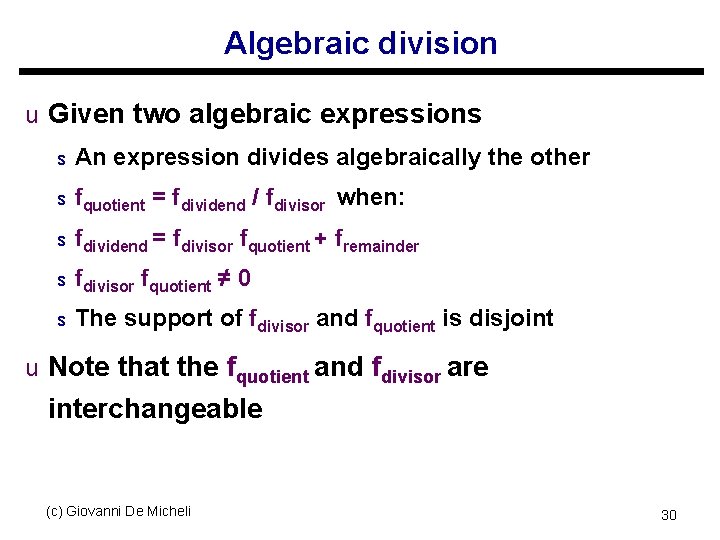
Algebraic division u Given two algebraic expressions s An expression divides algebraically the other s fquotient = fdividend / fdivisor when: s fdividend = fdivisor fquotient + fremainder s fdivisor fquotient s ≠ 0 The support of fdivisor and fquotient is disjoint u Note that the fquotient and fdivisor are interchangeable (c) Giovanni De Micheli 30

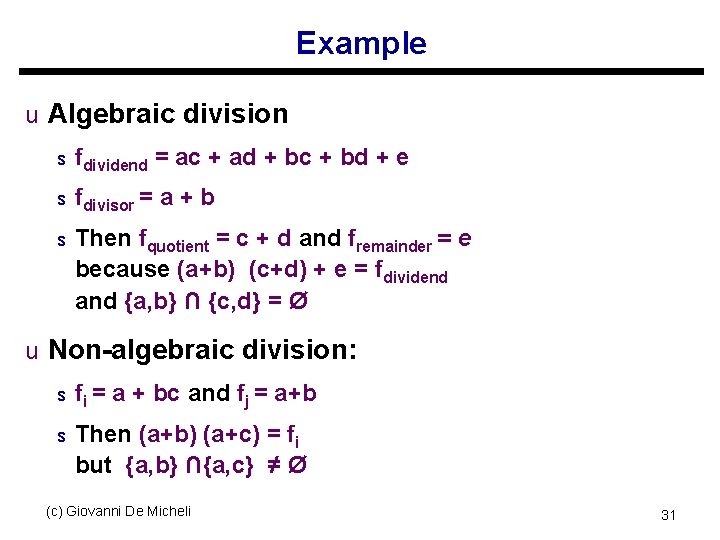
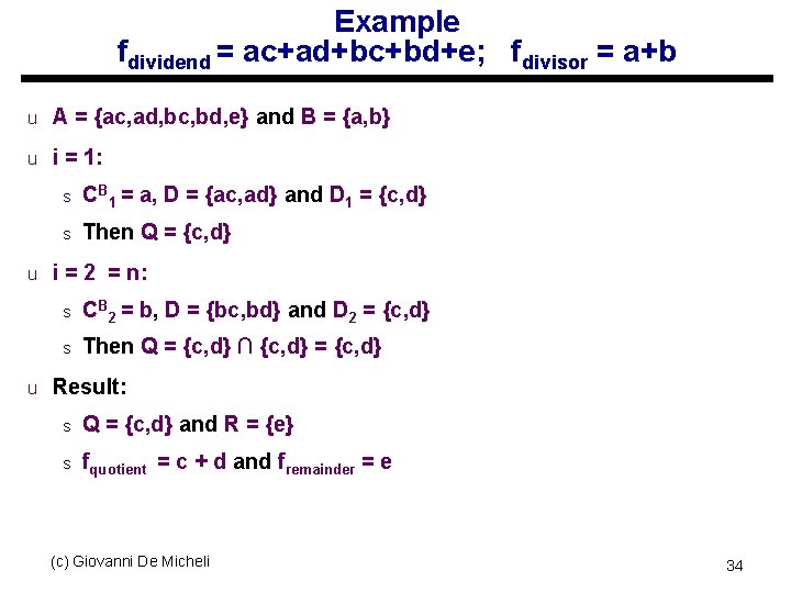
Example u Algebraic division s fdividend = ac + ad + bc + bd + e s fdivisor = a+b s Then fquotient = c + d and fremainder = e because (a+b) (c+d) + e = fdividend and {a, b} ∩ {c, d} = Ø u Non-algebraic division: s fi = s a + bc and fj = a+b Then (a+b) (a+c) = fi but {a, b} ∩{a, c} ≠ Ø (c) Giovanni De Micheli 31

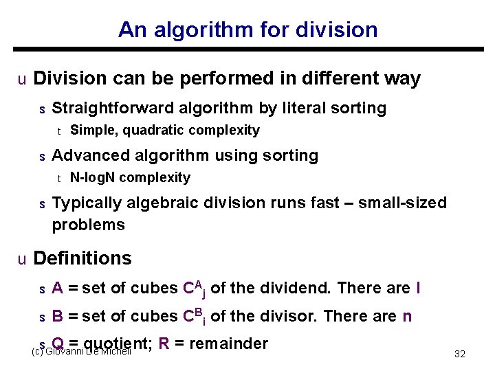
An algorithm for division u Division can be performed in different way s Straightforward algorithm by literal sorting t s Advanced algorithm using sorting t s Simple, quadratic complexity N-log. N complexity Typically algebraic division runs fast – small-sized problems u Definitions s A = set of cubes CAj of the dividend. There are l s B = set of cubes CBi of the divisor. There are n s Q = quotient; R = remainder (c) Giovanni De Micheli 32

Example fdividend = ac+ad+bc+bd+e; fdivisor = a+b u A = {ac, ad, bc, bd, e} and B = {a, b} u i = 1: s CB 1 = a, D = {ac, ad} and D 1 = {c, d} s Then Q = {c, d} u i = 2 = n: s CB 2 = b, D = {bc, bd} and D 2 = {c, d} s Then Q = {c, d} ∩ {c, d} = {c, d} u Result: s Q = {c, d} and R = {e} s fquotient = c + d and fremainder = e (c) Giovanni De Micheli 34

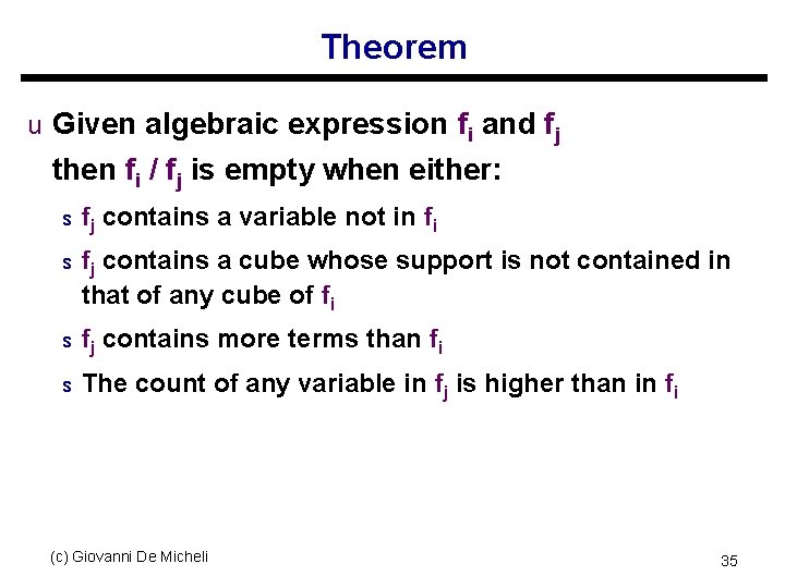
Theorem u Given algebraic expression fi and fj then fi / fj is empty when either: s fj contains a variable not in fi s fj contains a cube whose support is not contained in that of any cube of fi s fj s contains more terms than fi The count of any variable in fj is higher than in fi (c) Giovanni De Micheli 35

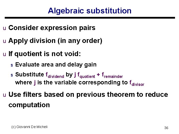
Algebraic substitution u Consider expression pairs u Apply division (in any order) u If quotient is not void: s Evaluate area and delay gain s Substitute fdividend by j fquotient + fremainder where j is the variable corresponding to fdivisor u Use filters based on previous theorem to reduce computation (c) Giovanni De Micheli 36

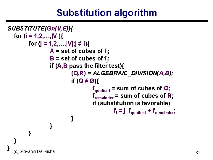
Substitution algorithm SUBSTITUTE(Gn(V, E)){ for (i = 1, 2, …, |V|){ for (j = 1, 2, …, |V|; j ≠ i){ A = set of cubes of fi; B = set of cubes of fj; if (A, B pass the filter test){ (Q, R) = ALGEBRAIC_DIVISION(A, B); if (Q ≠ Ø){ fquotient = sum of cubes of Q; fremainder = sum of cubes of R; if (substitution is favorable) fi = j fquotient + fremainder; } } } (c) Giovanni De Micheli 37

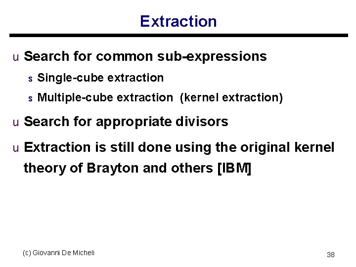
Extraction u Search for common sub-expressions s Single-cube extraction s Multiple-cube extraction (kernel extraction) u Search for appropriate divisors u Extraction is still done using the original kernel theory of Brayton and others [IBM] (c) Giovanni De Micheli 38

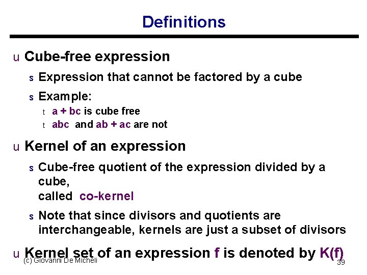
Definitions u Cube-free expression s Expression that cannot be factored by a cube s Example: t t a + bc is cube free abc and ab + ac are not u Kernel of an expression s Cube-free quotient of the expression divided by a cube, called co-kernel s Note that since divisors and quotients are interchangeable, kernels are just a subset of divisors u (c) Kernel set of an expression f is denoted by K(f) Giovanni De Micheli 39

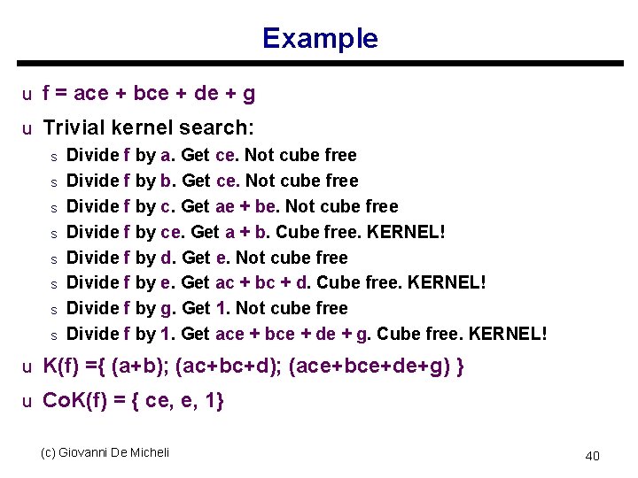
Example u f = ace + bce + de + g u Trivial kernel search: s Divide f by a. Get ce. Not cube free s Divide f by b. Get ce. Not cube free s Divide f by c. Get ae + be. Not cube free s Divide f by ce. Get a + b. Cube free. KERNEL! s Divide f by d. Get e. Not cube free s Divide f by e. Get ac + bc + d. Cube free. KERNEL! s Divide f by g. Get 1. Not cube free s Divide f by 1. Get ace + bce + de + g. Cube free. KERNEL! u K(f) ={ (a+b); (ac+bc+d); (ace+bce+de+g) } u Co. K(f) = { ce, e, 1} (c) Giovanni De Micheli 40

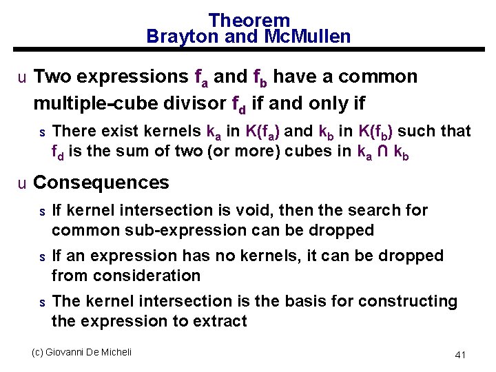
Theorem Brayton and Mc. Mullen u Two expressions fa and fb have a common multiple-cube divisor fd if and only if s There exist kernels ka in K(fa) and kb in K(fb) such that fd is the sum of two (or more) cubes in ka ∩ kb u Consequences s If kernel intersection is void, then the search for common sub-expression can be dropped s If an expression has no kernels, it can be dropped from consideration s The kernel intersection is the basis for constructing the expression to extract (c) Giovanni De Micheli 41

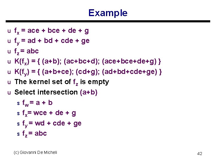
Example u fx = ace + bce + de + g u fy = ad + bd + cde + ge u fz = abc u K(fx) = { (a+b); (ac+bc+d); (ace+bce+de+g) } u K(fy) = { (a+b+ce); (cd+g); (ad+bd+cde+ge) } u The kernel set of fz is empty u Select intersection (a+b) s fw = s s s a+b fx= wce + de + g fy = wd + cde + ge fz = abc (c) Giovanni De Micheli 42

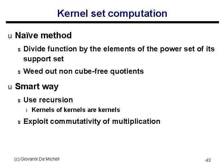
Kernel set computation u Naïve method s Divide function by the elements of the power set of its support set s Weed out non cube-free quotients u Smart way s Use recursion t s Kernels of kernels are kernels Exploit commutativity of multiplication (c) Giovanni De Micheli 43

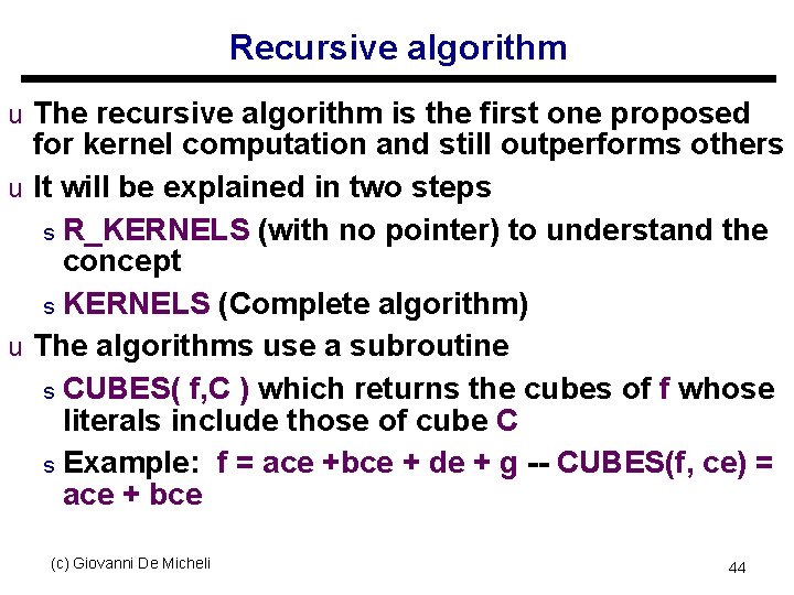
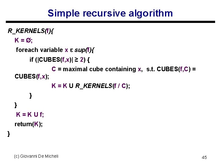
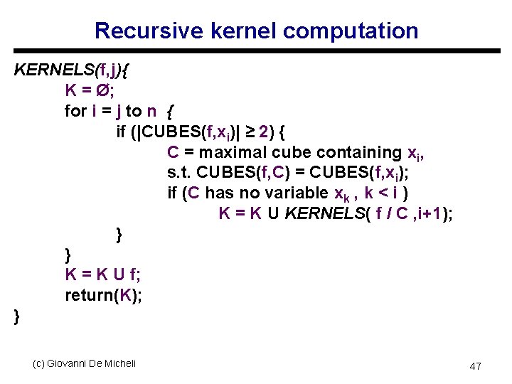
Recursive algorithm u The recursive algorithm is the first one proposed for kernel computation and still outperforms others u It will be explained in two steps s R_KERNELS (with no pointer) to understand the concept s KERNELS (Complete algorithm) u The algorithms use a subroutine s CUBES( f, C ) which returns the cubes of f whose literals include those of cube C s Example: f = ace +bce + de + g -- CUBES(f, ce) = ace + bce (c) Giovanni De Micheli 44

Simple recursive algorithm R_KERNELS(f){ K = Ø; foreach variable x ε sup(f){ if (|CUBES(f, x)| ≥ 2) { C = maximal cube containing x, s. t. CUBES(f, C) = CUBES(f, x); K = K U R_KERNELS(f / C); } } K = K U f; return(K); } (c) Giovanni De Micheli 45

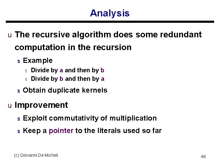
Analysis u The recursive algorithm does some redundant computation in the recursion s Example t t s Divide by a and then by b Divide by b and then by a Obtain duplicate kernels u Improvement s Exploit commutativity of multiplication s Keep a pointer to the literals used so far (c) Giovanni De Micheli 46

Recursive kernel computation KERNELS(f, j){ K = Ø; for i = j to n { if (|CUBES(f, xi)| ≥ 2) { C = maximal cube containing xi, s. t. CUBES(f, C) = CUBES(f, xi); if (C has no variable xk , k < i ) K = K U KERNELS( f / C , i+1); } } K = K U f; return(K); } (c) Giovanni De Micheli 47

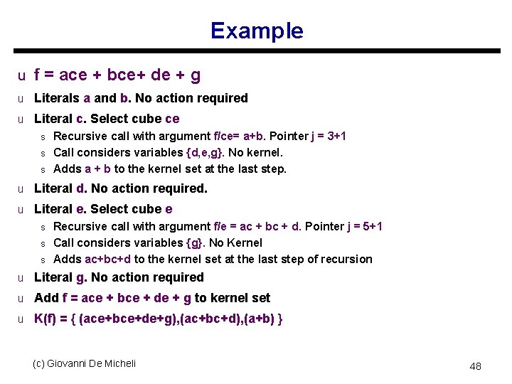
Example u f = ace + bce+ de + g u Literals a and b. No action required u Literal c. Select cube ce s s s Recursive call with argument f/ce= a+b. Pointer j = 3+1 Call considers variables {d, e, g}. No kernel. Adds a + b to the kernel set at the last step. u Literal d. No action required. u Literal e. Select cube e s s s Recursive call with argument f/e = ac + bc + d. Pointer j = 5+1 Call considers variables {g}. No Kernel Adds ac+bc+d to the kernel set at the last step of recursion u Literal g. No action required u Add f = ace + bce + de + g to kernel set u K(f) = { (ace+bce+de+g), (ac+bc+d), (a+b) } (c) Giovanni De Micheli 48

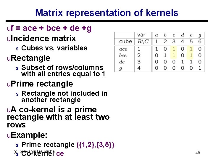
Matrix representation of kernels uf = ace + bce + de +g u. Incidence matrix s Cubes vs. variables u. Rectangle s Subset of rows/columns with all entries equal to 1 u. Prime rectangle s Rectangle not included in another rectangle u. A co-kernel is a prime rectangle with at least two rows u. Example: Prime rectangle ({1, 2}, {3, 5}) (c) Giovanni De Micheli s Co-kernel ce s 49

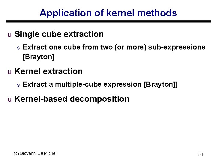
Application of kernel methods u Single cube extraction s Extract one cube from two (or more) sub-expressions [Brayton] u Kernel extraction s Extract a multiple-cube expression [Brayton]] u Kernel-based decomposition (c) Giovanni De Micheli 50

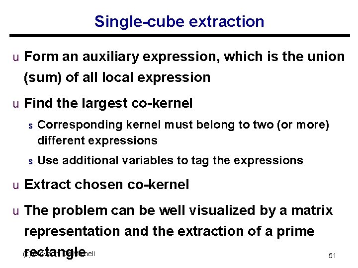
Single-cube extraction u Form an auxiliary expression, which is the union (sum) of all local expression u Find the largest co-kernel s Corresponding kernel must belong to two (or more) different expressions s Use additional variables to tag the expressions u Extract chosen co-kernel u The problem can be well visualized by a matrix representation and the extraction of a prime rectangle (c) Giovanni De Micheli 51

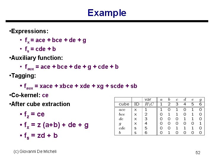
Example • Expressions: • fx = ace + bce + de + g • fs = cde + b • Auxiliary function: • faux = ace + bce + de + g + cde + b • Tagging: • faux = xace + xbce + xde + xg + scde + sb • Co-kernel: ce • After cube extraction • fz = ce • fx = z (a+b) + de + g • fs = zd + b (c) Giovanni De Micheli 52

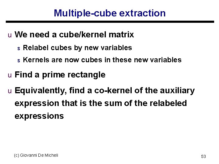
Multiple-cube extraction u We need a cube/kernel matrix s Relabel cubes by new variables s Kernels are now cubes in these new variables u Find a prime rectangle u Equivalently, find a co-kernel of the auxiliary expression that is the sum of the relabeled expressions (c) Giovanni De Micheli 53

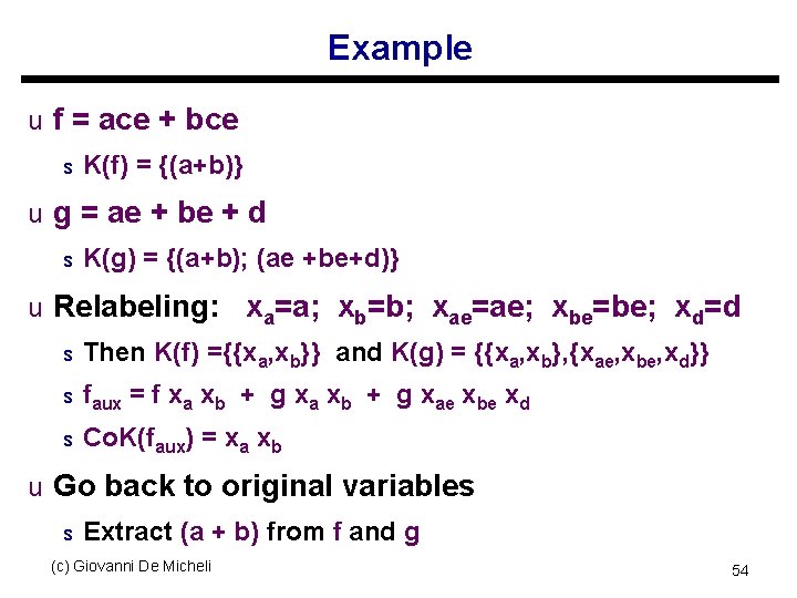
Example u f = ace + bce s K(f) = {(a+b)} u g = ae + be + d s K(g) = {(a+b); (ae +be+d)} u Relabeling: xa=a; xb=b; xae=ae; xbe=be; xd=d s Then K(f) ={{xa, xb}} and K(g) = {{xa, xb}, {xae, xbe, xd}} s faux s = f xa xb + g xae xbe xd Co. K(faux) = xa xb u Go back to original variables s Extract (a + b) from f and g (c) Giovanni De Micheli 54

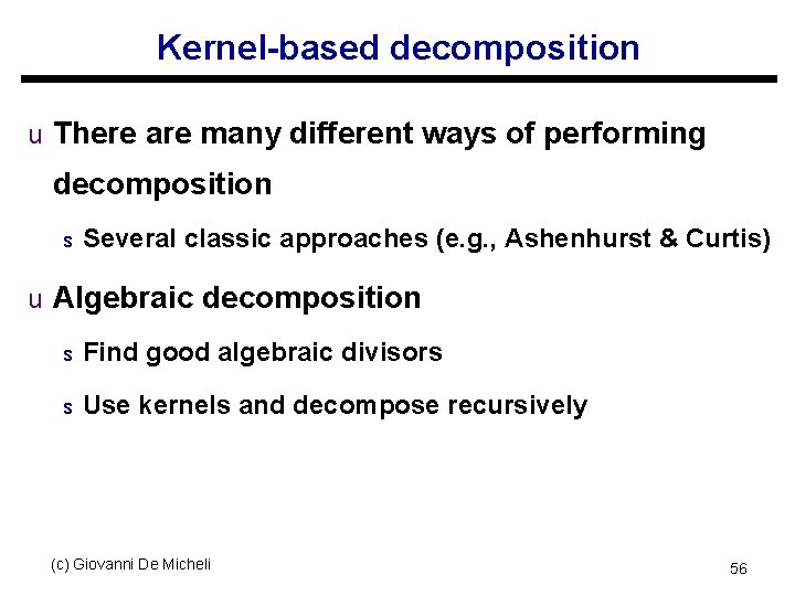
Kernel-based decomposition u There are many different ways of performing decomposition s Several classic approaches (e. g. , Ashenhurst & Curtis) u Algebraic decomposition s Find good algebraic divisors s Use kernels and decompose recursively (c) Giovanni De Micheli 56

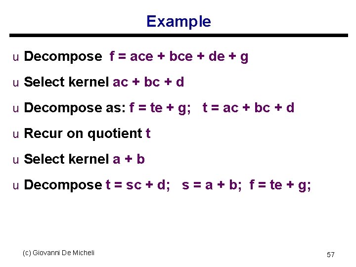
Example u Decompose f = ace + bce + de + g u Select kernel ac + bc + d u Decompose as: f = te + g; t = ac + bc + d u Recur on quotient t u Select kernel a + b u Decompose t = sc + d; s = a + b; f = te + g; (c) Giovanni De Micheli 57

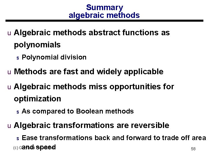
Summary algebraic methods u Algebraic methods abstract functions as polynomials s Polynomial division u Methods are fast and widely applicable u Algebraic methods miss opportunities for optimization s As compared to Boolean methods u Algebraic transformations are reversible Ease transformations back and forward to trade off area (c) Giovanni De Micheli and speed 58 s