Multilevel Analysis Kate Pickett Senior Lecturer in Epidemiology

Multilevel Analysis Kate Pickett Senior Lecturer in Epidemiology

Perspective ¢ Health researchers: Are interested in answering research questions (not maths) l Want to be able to apply statistical techniques l Want to be able to interpret results l Want to be able to communicate with consumers and statisticians l

Aims for this session Understand the rationale for multilevel analysis ¢ Understand common terminology ¢ Interpret output from multilevel models ¢ Be able to read and critically appraise studies using multilevel models ¢

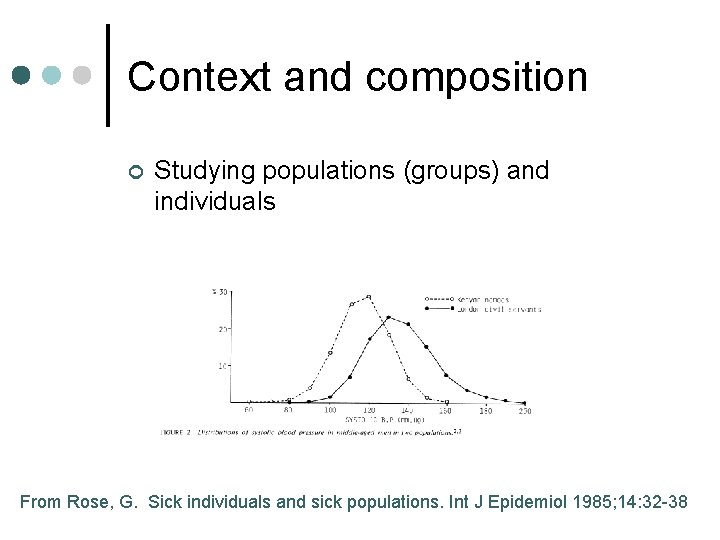
Context and composition ¢ Studying populations (groups) and individuals From Rose, G. Sick individuals and sick populations. Int J Epidemiol 1985; 14: 32 -38

Levels of analysis ¢ Health researchers may collect and use data collected at the level of: Individuals, patients l Families or other social groupings l Clinics or hospitals l Small areas, neighbourhoods l Large populations l

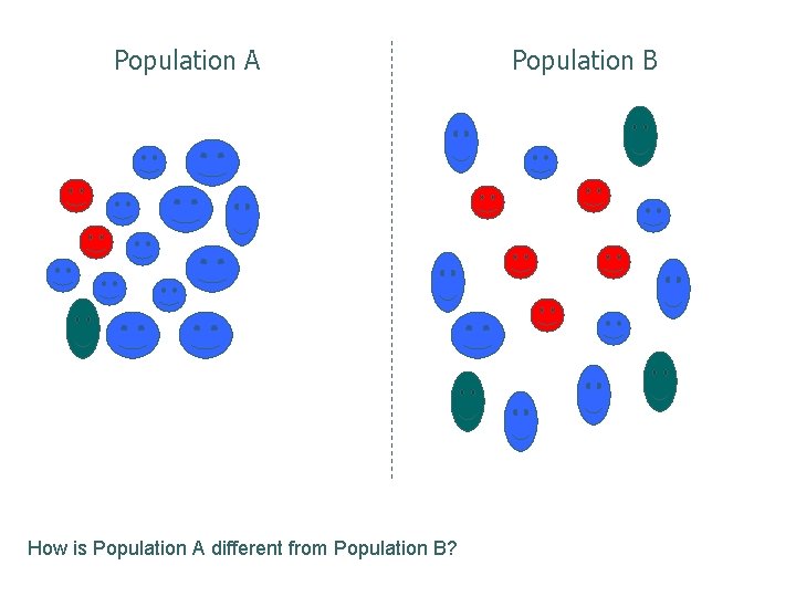
Population A How is Population A different from Population B? Population B

Ecological studies ¢ ¢ ¢ Data are aggregated and represent a group, rather than an individual l incidence rate of an illness l prevalence of a particular health service We don’t know which particular individuals within the group were ill or received the service These group-based outcome measures are analyzed by correlating them with determinants measured for the same groups

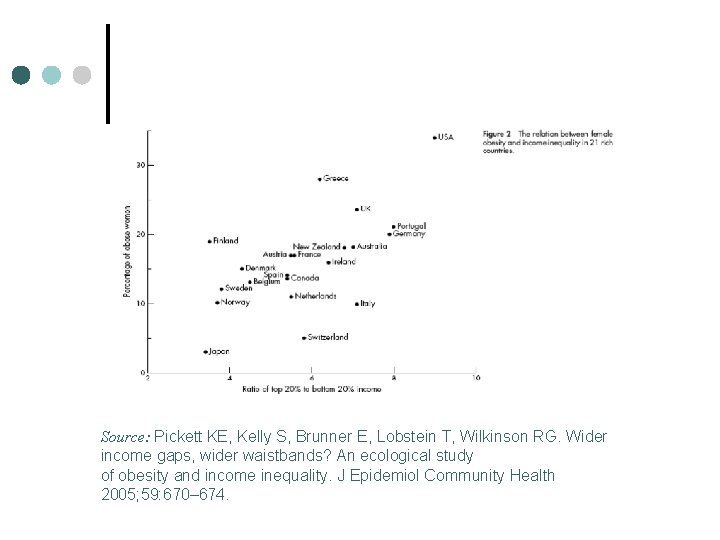
Source: Pickett KE, Kelly S, Brunner E, Lobstein T, Wilkinson RG. Wider income gaps, wider waistbands? An ecological study of obesity and income inequality. J Epidemiol Community Health 2005; 59: 670– 674.

The ecological fallacy ¢ ¢ Associations at the group level may not hold at an individual level l Eg, we might see that rates of obesity are correlated internationally with per capita calorie intake l But, we don’t know if it is the obese individuals who are eating all the calories Many group-level variables are correlated so we may get spurious correlations l Eg, obesity rates may also be correlated with number of zoos per capita or some other completely unrelated factor

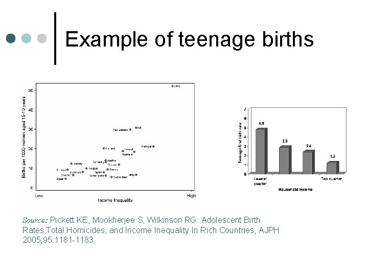
The atomistic fallacy ¢ But the ecological fallacy has a flip side l Factors that affect outcomes in individuals may not operate in the same way at the population level • Eg, teenage births are more common among the poor, but teenage birth rates are very high in some very wealthy countries.

Example of teenage births Source: Pickett KE, Mookherjee S, Wilkinson RG. Adolescent Birth Rates, Total Homicides, and Income Inequality In Rich Countries, AJPH 2005; 95: 1181 -1183.

Ecological variables ¢ ¢ Sometimes ecological studies are done because it is quick and easy Sometimes ecological studies are the best design for the research question BECAUSE ¢ Some determinants are “ecological”: l l l Population density Air quality/pollution GNP Income inequality % unemployed Ambient temperature

Context and composition But what if we are interested in both types of variables (individual and population) simultaneously? ¢ Eg: we might want to know about the effect of population-level unemployment on health, above and beyond the health impact of being unemployed for any given individual ¢

Multilevel models

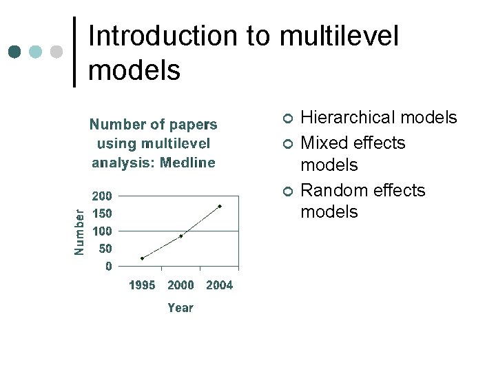
Introduction to multilevel models ¢ ¢ ¢ Hierarchical models Mixed effects models Random effects models

Background ¢ ¢ ¢ Developed in education research Observations of students in a single class are not independent of one another “Standard” statistical models assume that observations are independent ¢ Two-level hierarchy l ¢ Three-level hierarchy l ¢ Students within classes within schools Four-level hierarchy l Students within classes within schools within local authority areas

Health research context Patients within a medical practice ¢ Residents within neighbourhoods ¢ Subjects within trial clusters ¢ Hospitals within PCTs…. ¢

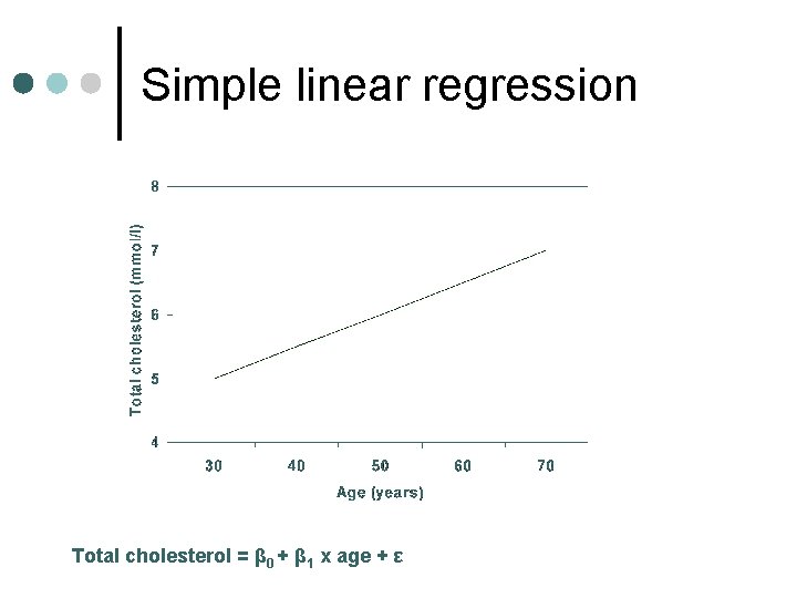
Examples for class ¢ ¢ Some examples are drawn from Twisk JWR “Applied Multilevel Analysis” Cambridge University Press, 2006 Example data are available at: http: www. emgo. nlresearchtools Research question: what is the relationship between total cholesterol and age? Statistical software: Stata but note that MLwi. N is free to UK academics: http: //www. cmm. bristol. ac. uk/MLwi. N/downlo ad/index. shtml)

Simple linear regression Total cholesterol = β 0 + β 1 x age + ε

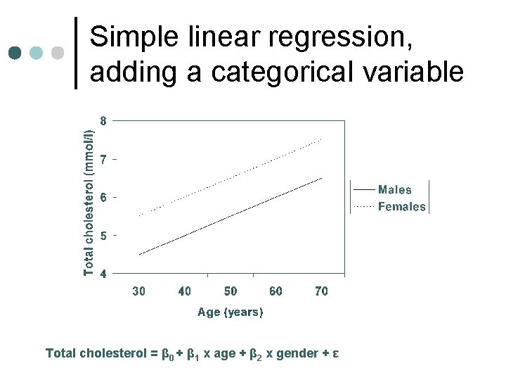
Simple linear regression, adding a categorical variable Total cholesterol = β 0 + β 1 x age + β 2 x gender + ε

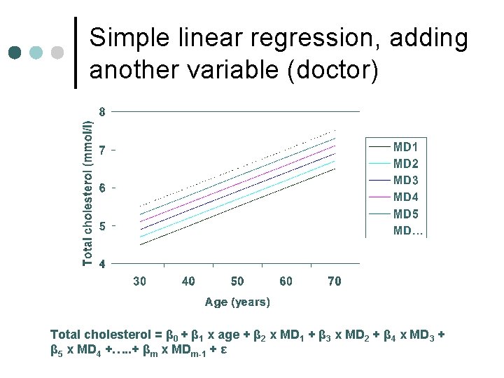
Simple linear regression, adding another variable (doctor) Total cholesterol = β 0 + β 1 x age + β 2 x MD 1 + β 3 x MD 2 + β 4 x MD 3 + β 5 x MD 4 +…. . + βm x MDm-1 + ε

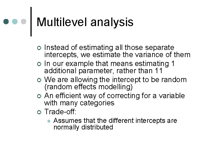
Multilevel analysis ¢ ¢ ¢ Instead of estimating all those separate intercepts, we estimate the variance of them In our example that means estimating 1 additional parameter, rather than 11 We are allowing the intercept to be random (random effects modelling) An efficient way of correcting for a variable with many categories Trade-off: l Assumes that the different intercepts are normally distributed

Example data Cholesterol Dataset ¢ 441 patients ¢ Age 44 -86 years ¢ Cholesterol 3. 908. 86 mmol/l ¢ 12 doctors

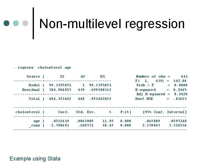
Non-multilevel regression . regress cholesterol age Source | SS df MS -------+---------------Model | 99. 3395851 1 99. 3395851 Residual | 306. 984057 439. 699280312 -------+---------------Total | 406. 323642 440. 923462822 Number of obs F( 1, 439) Prob > F R-squared Adj R-squared Root MSE = 441 = 142. 06 = 0. 0000 = 0. 2445 = 0. 2428 =. 83623 ---------------------------------------cholesterol | Coef. Std. Err. t P>|t| [95% Conf. Interval] -------+--------------------------------age |. 0512619. 0043009 11. 92 0. 000. 042809. 0597148 _cons | 2. 798691. 268571 10. 42 0. 000 2. 270847 3. 326536 --------------------------------------- Example using Stata

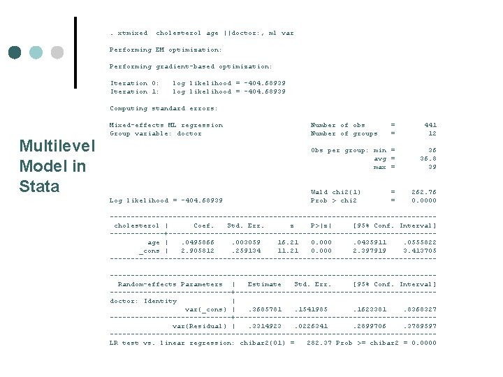
. xtmixed cholesterol age ||doctor: , ml var Performing EM optimization: Performing gradient-based optimization: Iteration 0: Iteration 1: log likelihood = -404. 68939 Computing standard errors: Multilevel Model in Stata Mixed-effects ML regression Group variable: doctor Log likelihood = -404. 68939 Number of obs Number of groups = = 441 12 Obs per group: min = avg = max = 36 36. 8 39 Wald chi 2(1) Prob > chi 2 = = 262. 76 0. 0000 ---------------------------------------cholesterol | Coef. Std. Err. z P>|z| [95% Conf. Interval] -------+--------------------------------age |. 0495866. 003059 16. 21 0. 000. 0435911. 0555822 _cons | 2. 905812. 259134 11. 21 0. 000 2. 397919 3. 413705 -----------------------------------------------------------------------------Random-effects Parameters | Estimate Std. Err. [95% Conf. Interval] ---------------+------------------------doctor: Identity | var(_cons) |. 3685781. 1541985. 1623381. 8368327 ---------------+------------------------var(Residual) |. 3314923. 0226341. 2899706. 3789597 ---------------------------------------LR test vs. linear regression: chibar 2(01) = 282. 37 Prob >= chibar 2 = 0. 0000

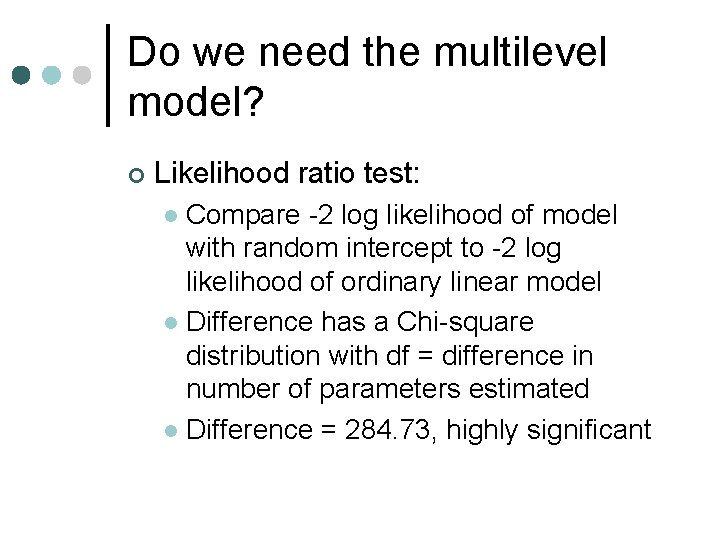
Do we need the multilevel model? ¢ Likelihood ratio test: Compare -2 log likelihood of model with random intercept to -2 log likelihood of ordinary linear model l Difference has a Chi-square distribution with df = difference in number of parameters estimated l Difference = 284. 73, highly significant l

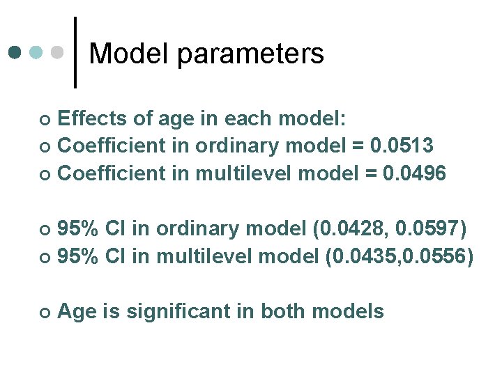
Model parameters Effects of age in each model: ¢ Coefficient in ordinary model = 0. 0513 ¢ Coefficient in multilevel model = 0. 0496 ¢ 95% CI in ordinary model (0. 0428, 0. 0597) ¢ 95% CI in multilevel model (0. 0435, 0. 0556) ¢ ¢ Age is significant in both models

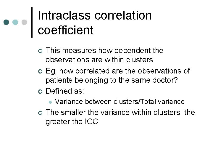
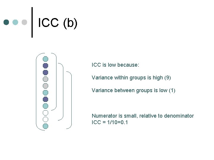
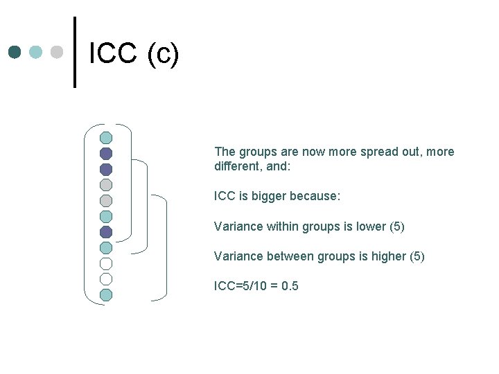
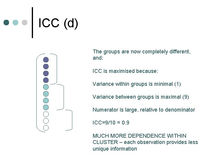
Intraclass correlation coefficient ¢ ¢ ¢ This measures how dependent the observations are within clusters Eg, how correlated are the observations of patients belonging to the same doctor? Defined as: l ¢ Variance between clusters/Total variance The smaller the variance within clusters, the greater the ICC

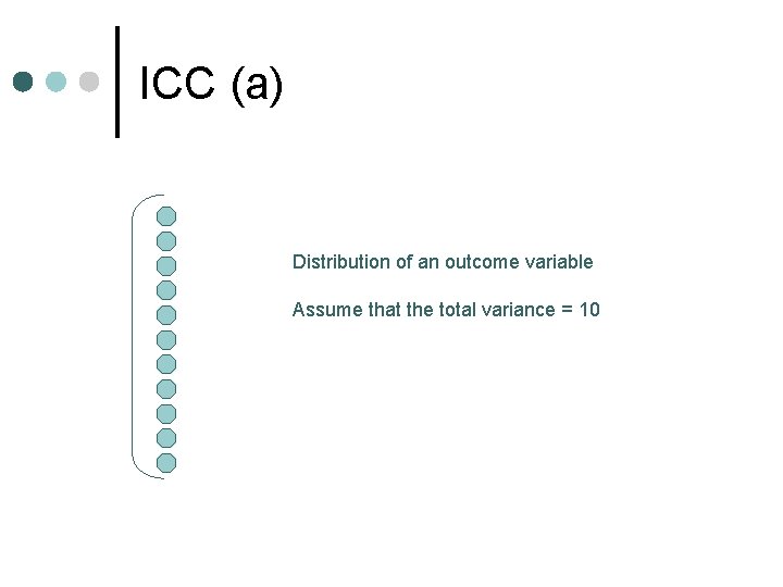
ICC (a) Distribution of an outcome variable Assume that the total variance = 10

ICC (b) ICC is low because: Variance within groups is high (9) Variance between groups is low (1) Numerator is small, relative to denominator ICC = 1/10=0. 1

ICC (c) The groups are now more spread out, more different, and: ICC is bigger because: Variance within groups is lower (5) Variance between groups is higher (5) ICC=5/10 = 0. 5

ICC (d) The groups are now completely different, and: ICC is maximised because: Variance within groups is minimal (1) Variance between groups is maximal (9) Numerator is large, relative to denominator ICC=9/10 = 0. 9 MUCH MORE DEPENDENCE WITHIN CLUSTER – each observation provides less unique information

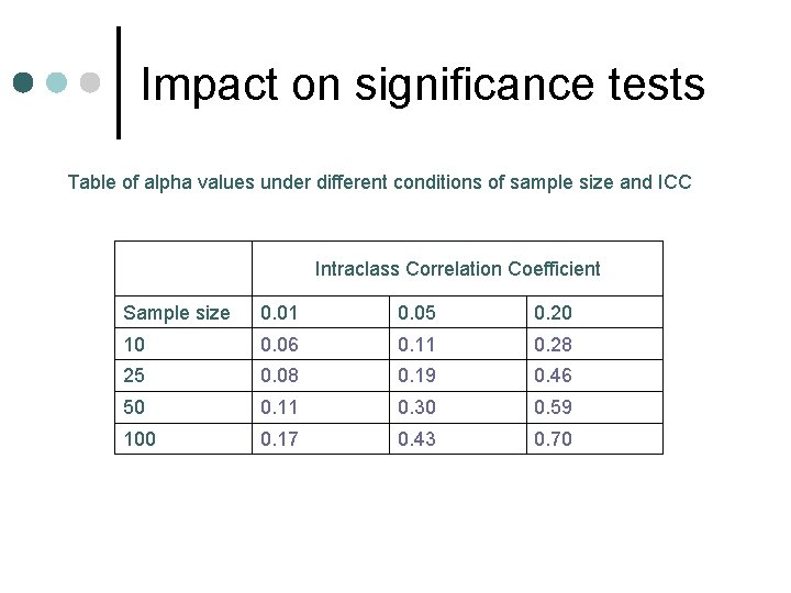
Impact on significance tests Table of alpha values under different conditions of sample size and ICC Intraclass Correlation Coefficient Sample size 0. 01 0. 05 0. 20 10 0. 06 0. 11 0. 28 25 0. 08 0. 19 0. 46 50 0. 11 0. 30 0. 59 100 0. 17 0. 43 0. 70

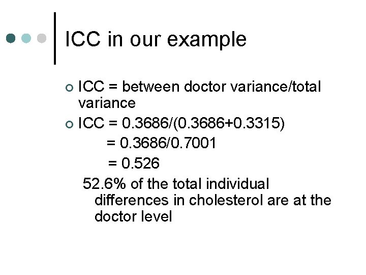
ICC in our example ICC = between doctor variance/total variance ¢ ICC = 0. 3686/(0. 3686+0. 3315) = 0. 3686/0. 7001 = 0. 526 52. 6% of the total individual differences in cholesterol are at the doctor level ¢

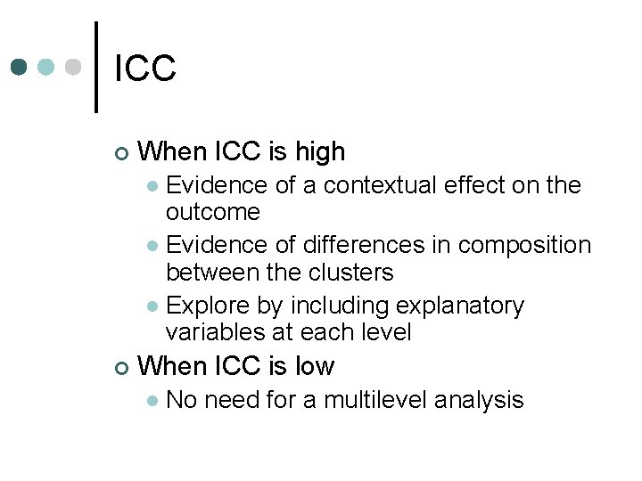
ICC ¢ When ICC is high Evidence of a contextual effect on the outcome l Evidence of differences in composition between the clusters l Explore by including explanatory variables at each level l ¢ When ICC is low l No need for a multilevel analysis

Back to unemployment example

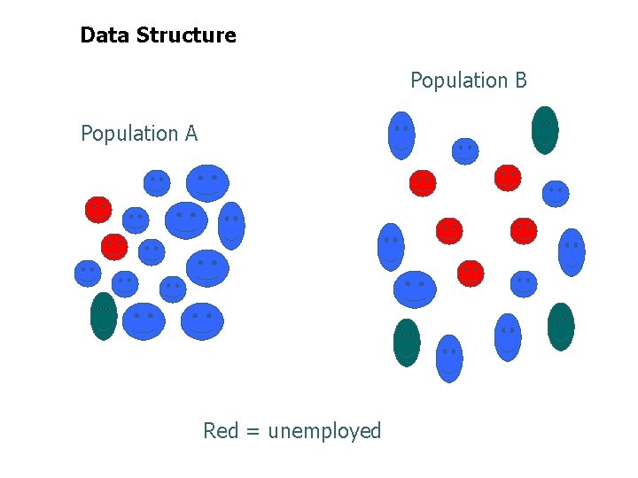
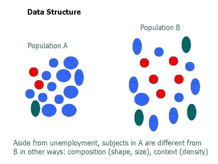
Data Structure Population B Population A Red = unemployed

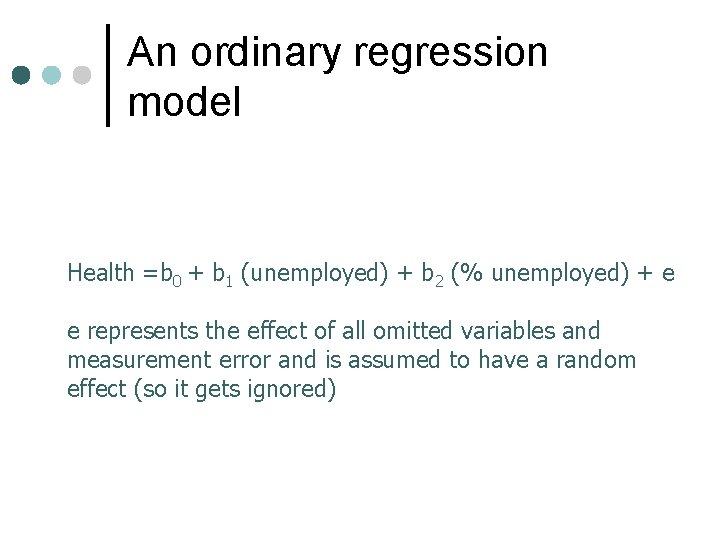
An ordinary regression model Health =b 0 + b 1 (unemployed) + b 2 (% unemployed) + e e represents the effect of all omitted variables and measurement error and is assumed to have a random effect (so it gets ignored)

Data Structure Population B Population A Aside from unemployment, subjects in A are different from B in other ways: composition (shape, size), context (density)

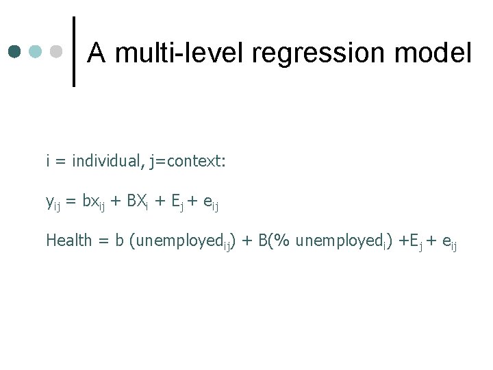
A multi-level regression model i = individual, j=context: yij = bxij + BXi + Ej + eij Health = b (unemployedij) + B(% unemployedi) +Ej + eij

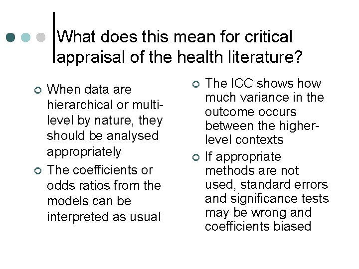
What does this mean for critical appraisal of the health literature? ¢ ¢ When data are hierarchical or multilevel by nature, they should be analysed appropriately The coefficients or odds ratios from the models can be interpreted as usual ¢ ¢ The ICC shows how much variance in the outcome occurs between the higherlevel contexts If appropriate methods are not used, standard errors and significance tests may be wrong and coefficients biased

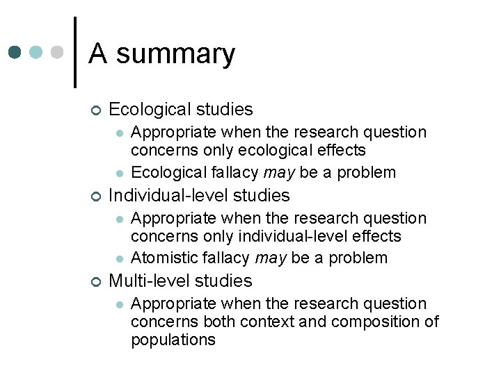
A summary ¢ Ecological studies l l ¢ Individual-level studies l l ¢ Appropriate when the research question concerns only ecological effects Ecological fallacy may be a problem Appropriate when the research question concerns only individual-level effects Atomistic fallacy may be a problem Multi-level studies l Appropriate when the research question concerns both context and composition of populations