Multilayer perceptron Usman Roshan Perceptron Gradient descent Perceptron

Multi-layer perceptron Usman Roshan

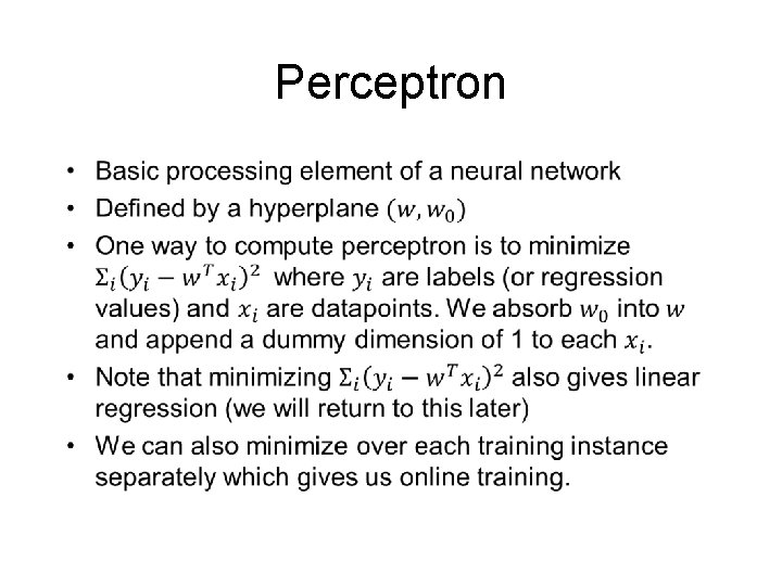
Perceptron •

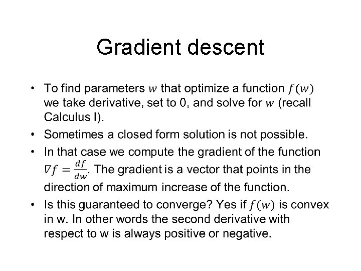
Gradient descent •

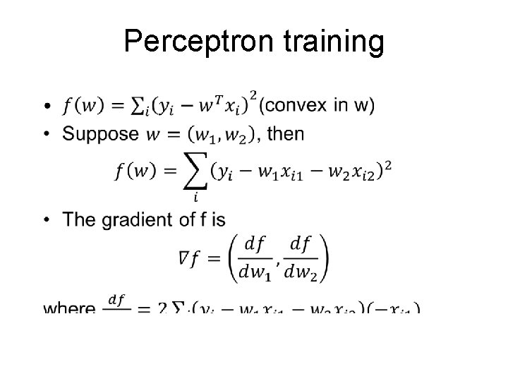
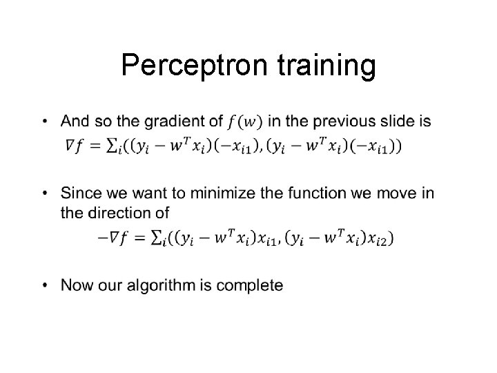
Perceptron training •

Perceptron training •

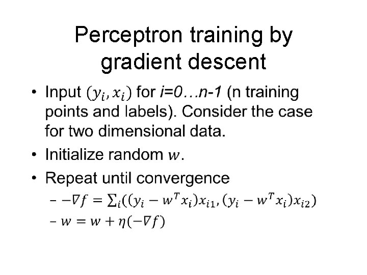
Perceptron training by gradient descent •

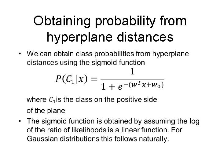
Obtaining probability from hyperplane distances •

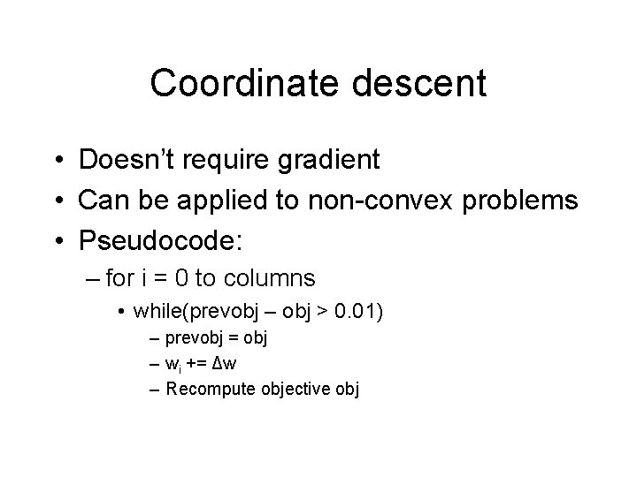
Coordinate descent • Doesn’t require gradient • Can be applied to non-convex problems • Pseudocode: – for i = 0 to columns • while(prevobj – obj > 0. 01) – prevobj = obj – wi += Δw – Recompute objective obj

Coordinate descent • Challenges with coordinate descent – Local minima with non-convex problems • How to escape local minima: – Random restarts – Simulated annealing – Iterated local search

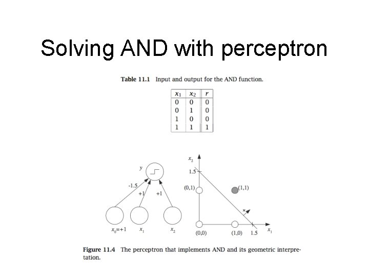
Solving AND with perceptron

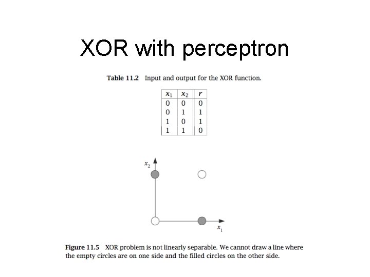
XOR with perceptron

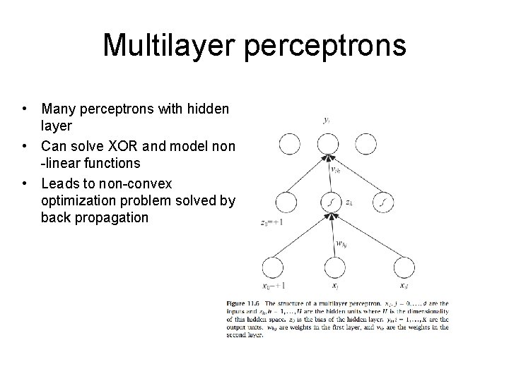
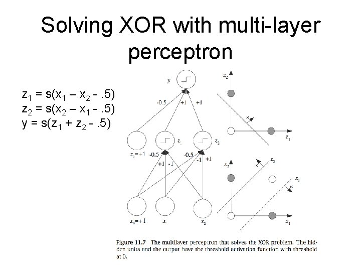
Multilayer perceptrons • Many perceptrons with hidden layer • Can solve XOR and model non -linear functions • Leads to non-convex optimization problem solved by back propagation

Solving XOR with multi-layer perceptron z 1 = s(x 1 – x 2 -. 5) z 2 = s(x 2 – x 1 -. 5) y = s(z 1 + z 2 -. 5)

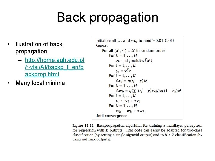
Back propagation • Ilustration of back propagation – http: //home. agh. edu. pl /~vlsi/AI/backp_t_en/b ackprop. html • Many local minima

Training issues for multilayer perceptrons • Convergence rate – Momentum • Adaptive learning • Overtraining – Early stopping

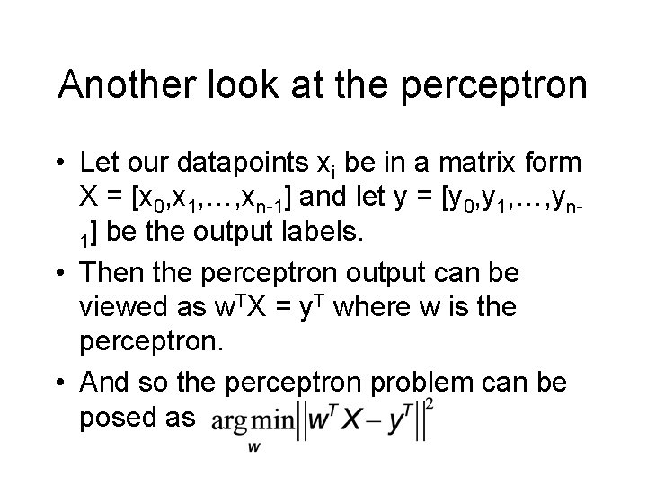
Another look at the perceptron • Let our datapoints xi be in a matrix form X = [x 0, x 1, …, xn-1] and let y = [y 0, y 1, …, yn 1] be the output labels. • Then the perceptron output can be viewed as w. TX = y. T where w is the perceptron. • And so the perceptron problem can be posed as

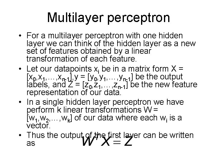
Multilayer perceptron • For a multilayer perceptron with one hidden layer we can think of the hidden layer as a new set of features obtained by a linear transformation of each feature. • Let our datapoints xi be in a matrix form X = [x 0, x 1, …, xn-1], y = [y 0, y 1, …, yn-1] be the output labels, and Z = [z 0, z 1, …, zn-1] be the new feature representation of our data. • In a single hidden layer perceptron we have perform k linear transformations W = [w 1, w 2, …, wk] of our data where each wi is a vector. • Thus the output of the first layer can be written as

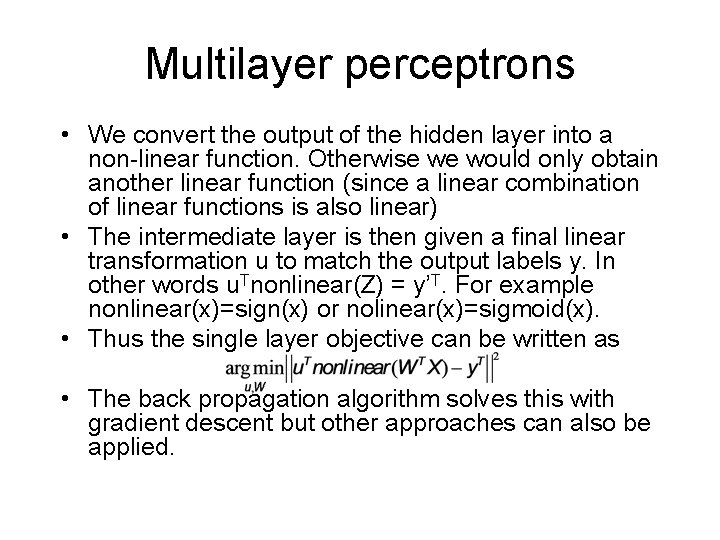
Multilayer perceptrons • We convert the output of the hidden layer into a non-linear function. Otherwise we would only obtain another linear function (since a linear combination of linear functions is also linear) • The intermediate layer is then given a final linear transformation u to match the output labels y. In other words u. Tnonlinear(Z) = y’T. For example nonlinear(x)=sign(x) or nolinear(x)=sigmoid(x). • Thus the single layer objective can be written as • The back propagation algorithm solves this with gradient descent but other approaches can also be applied.