Multifactorial traits and complex genetics I Genomewide association

- Slides: 65

Multifactorial traits and complex genetics I Genome-wide association studies in humans gavin. band@well. ox. ac. uk Wellcome Centre for Human Genetics

Overview Describe studies aiming to find genetic differences between individuals that influence susceptibility to diseases (or other traits).

Objectives * What does it mean to ‘find disease genes’? * Learn about study designs that look for genetic differences between individuals that underlie complex phenotypes - like diseases. * Appreciate some of the practical and theoretical complexities of these studies.

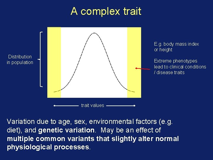
A complex trait E. g. body mass index or height Distribution in population Extreme phenotypes lead to clinical conditions / disease traits trait values Variation due to age, sex, environmental factors (e. g. diet), and genetic variation. May be an effect of multiple common variants that slightly alter normal physiological processes.

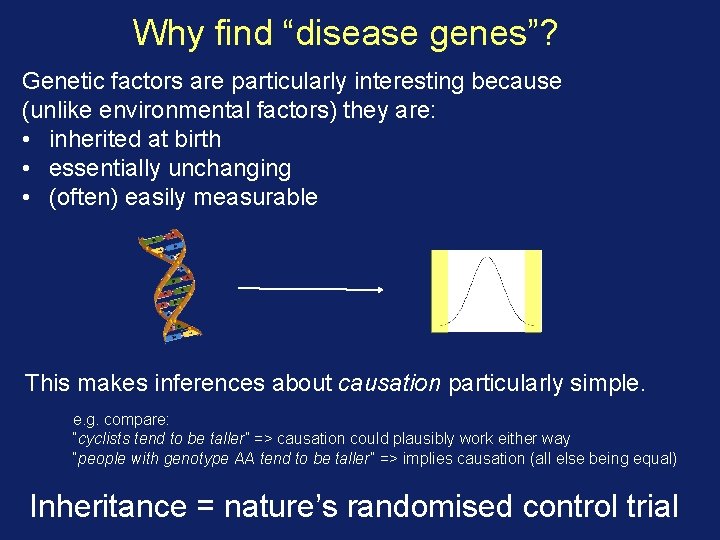
Why find “disease genes”? Genetic factors are particularly interesting because (unlike environmental factors) they are: • inherited at birth • essentially unchanging • (often) easily measurable This makes inferences about causation particularly simple. e. g. compare: “cyclists tend to be taller” => causation could plausibly work either way “people with genotype AA tend to be taller” => implies causation (all else being equal) Inheritance = nature’s randomised control trial

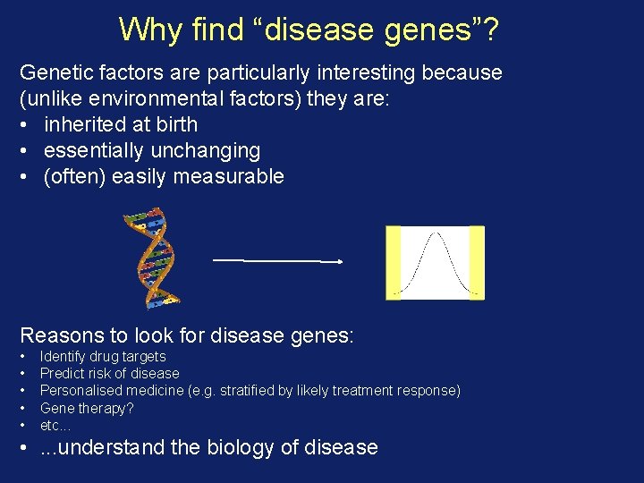
Why find “disease genes”? Genetic factors are particularly interesting because (unlike environmental factors) they are: • inherited at birth • essentially unchanging • (often) easily measurable Reasons to look for disease genes: • • • Identify drug targets Predict risk of disease Personalised medicine (e. g. stratified by likely treatment response) Gene therapy? etc. . . • . . . understand the biology of disease

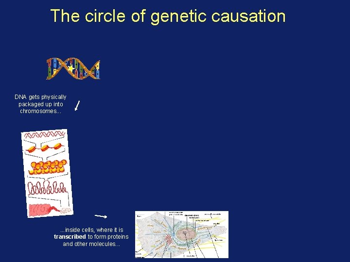
The circle of genetic causation (a causal mutation)

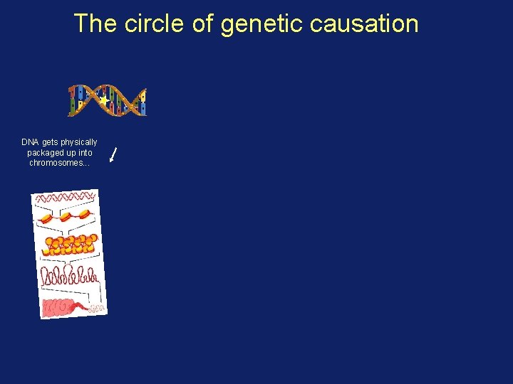
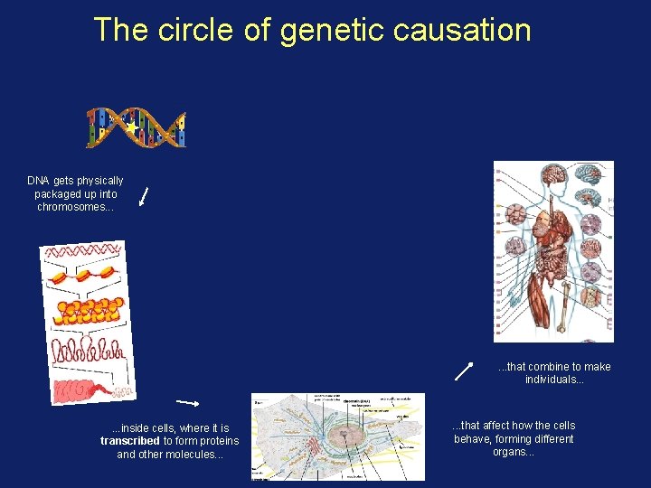
The circle of genetic causation DNA gets physically packaged up into chromosomes. . .

The circle of genetic causation DNA gets physically packaged up into chromosomes. . . inside cells, where it is transcribed to form proteins and other molecules. . .

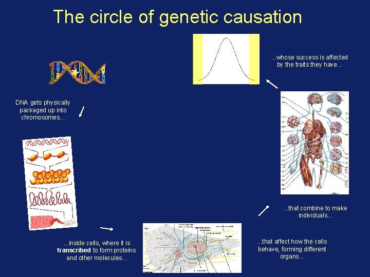
The circle of genetic causation DNA gets physically packaged up into chromosomes. . . that combine to make individuals. . . inside cells, where it is transcribed to form proteins and other molecules. . . that affect how the cells behave, forming different organs. . .

The circle of genetic causation. . . whose success is affected by the traits they have. . . DNA gets physically packaged up into chromosomes. . . that combine to make individuals. . . inside cells, where it is transcribed to form proteins and other molecules. . . that affect how the cells behave, forming different organs. . .

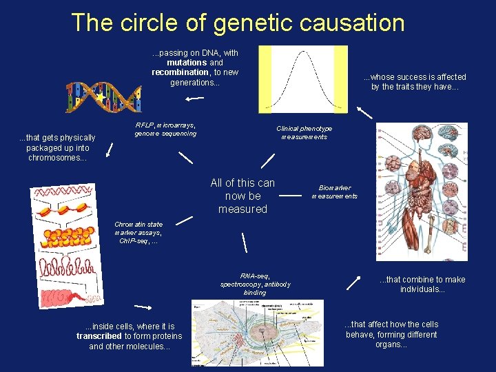
The circle of genetic causation. . . passing on DNA, with mutations and recombination, to new generations. . . whose success is affected by the traits they have. . . that gets physically packaged up into chromosomes. . . that combine to make individuals. . . inside cells, where it is transcribed to form proteins and other molecules. . . that affect how the cells behave, forming different organs. . .

The circle of genetic causation. . . passing on DNA, with mutations and recombination, to new generations. . . that gets physically packaged up into chromosomes. . . RFLP, microarrays, genome sequencing . . . whose success is affected by the traits they have. . . Clinical phenotype measurements All of this can now be measured Biomarker measurements Chromatin state marker assays, Ch. IP-seq, . . . RNA-seq, spectroscopy, antibody binding . . . inside cells, where it is transcribed to form proteins and other molecules. . . that combine to make individuals. . . that affect how the cells behave, forming different organs. . .

Summary 1 It is clinically useful and interesting to look for the genetic variants contributing to complex human traits The mapping of genetics to traits is likely to be complex because of the complex / interesting processes involved. Now’s an exciting time to be working on this - we now have the technology to attack it at large scale.

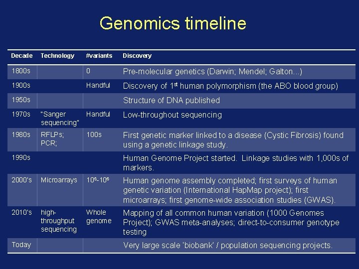
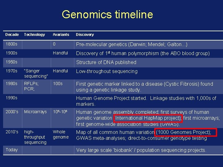
Genomics timeline Decade Technology #variants Discovery 1800 s 0 Pre-molecular genetics (Darwin; Mendel; Galton. . . ) 1900 s Handful Discovery of 1 st human polymorphism (the ABO blood group) 1950 s Structure of DNA published 1970 s “Sanger sequencing” Handful Low-throughout sequencing 1980 s RFLPs; PCR; 100 s First genetic marker linked to a disease (Cystic Fibrosis) found using a genetic linkage study. 1990 s Human Genome Project started. Linkage studies with 1, 000 s of markers. 2000’s Microarrays 105 -106 Human genome assembly completed; first surveys of human genetic variation (International Hap. Map project); first microarrays; first genome-wide association studies (GWAS). 2010’s highthroughput sequencing Whole genome Mapping of all common human variation (1000 Genomes Project); GWAS meta-analyses; direct-to-consumer genotype testing Today Very large scale ‘biobank’ / population sequencing projects.

Finding disease genes in practice

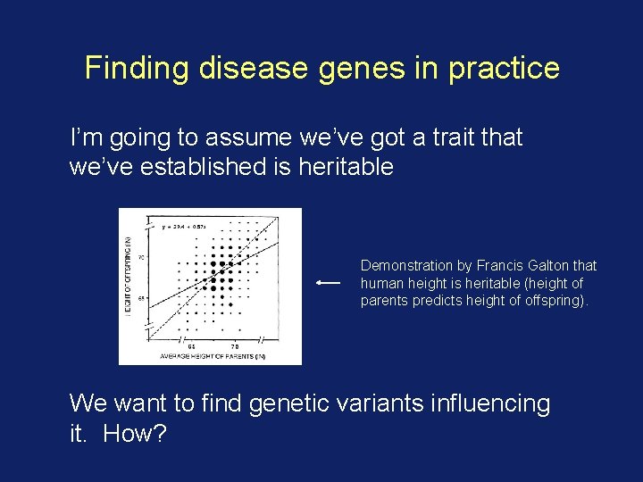
Finding disease genes in practice I’m going to assume we’ve got a trait that we’ve established is heritable Demonstration by Francis Galton that human height is heritable (height of parents predicts height of offspring). We want to find genetic variants influencing it. How?

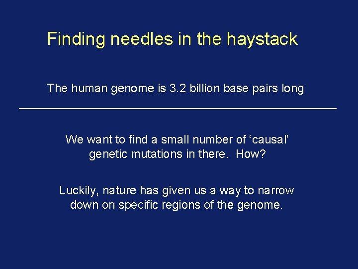
Finding needles in the haystack The human genome is 3. 2 billion base pairs long We want to find a small number of ‘causal’ genetic mutations in there. How? Luckily, nature has given us a way to narrow down on specific regions of the genome.

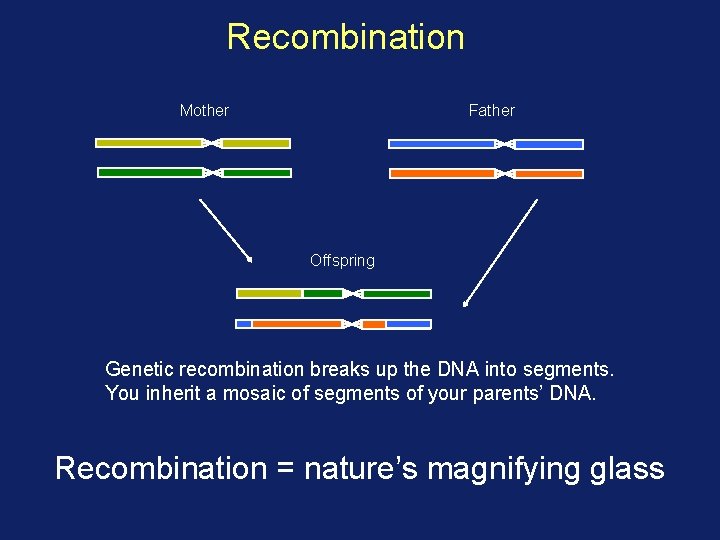
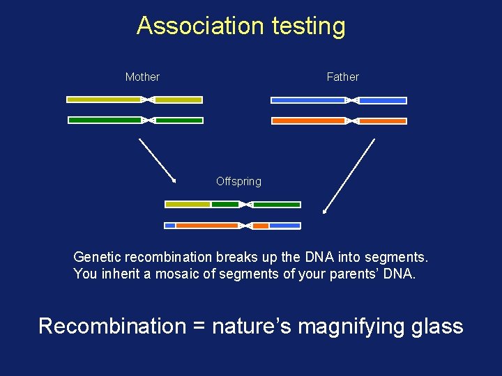
Recombination Mother Father Offspring Genetic recombination breaks up the DNA into segments. You inherit a mosaic of segments of your parents’ DNA. Recombination = nature’s magnifying glass

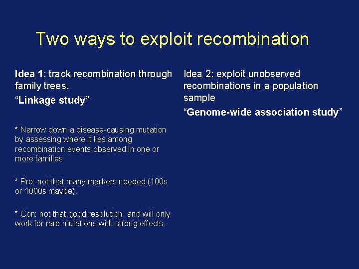
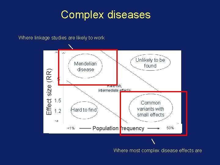
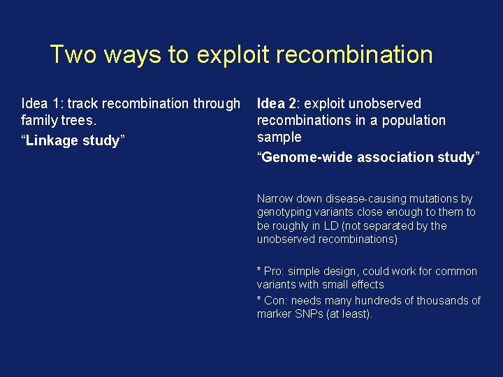
Two ways to exploit recombination Idea 1: track recombination through family trees. “Linkage study” * Narrow down a disease-causing mutation by assessing where it lies among recombination events observed in one or more families * Pro: not that many markers needed (100 s or 1000 s maybe). * Con: not that good resolution, and will only work for rare mutations with strong effects. Idea 2: exploit unobserved recombinations in a population sample “Genome-wide association study”

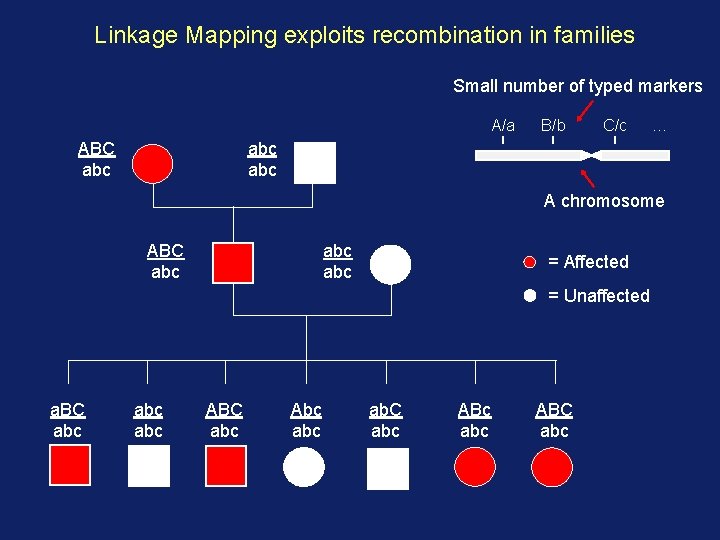
Linkage Mapping exploits recombination in families Small number of typed markers A/a ABC abc B/b C/c … abc A chromosome ABC abc abc = Affected = Unaffected a. BC abc abc ABC abc Abc ab. C abc ABc abc ABC abc

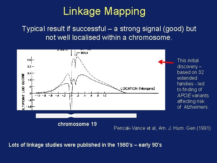
Linkage Mapping Typical result if successful – a strong signal (good) but not well localised within a chromosome. This initial discovery – based on 32 extended families - led to finding of APOE variants affecting risk of Alzheimers. chromosome 19 Pericak-Vance et al, Am. J. Hum. Gen (1991) Lots of linkage studies were published in the 1980’s – early 90’s

Successes and Failures circa 2000 Linkage Mapping was successful in identifying the genetic basis of many human diseases in which the disease penetrance resembles a simple Mendelian model e. g. Huntington’s disease (HD 1993), Cystic Fibrosis, some forms of breast cancer (BRCA 1 1993), Alzheimers (APOE 1991)… But “the literature is now replete with linkage screens for an array of common ‘complex’ disorders such as schizophrenia, manic depression, autism, asthma, type I and type II diabetes, Multiple Sclerosis, Lupus. Although many of these studies have reported significant linkage findings, none has lead to convincing replication” – Risch (2000)

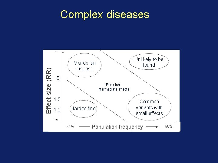
Relative risk measures the chance of getting disease if exposed to the risk genotype, versus the chance if not exposed: Relative risk = P( disease | carry risk allele ) P( disease | don’t carry the risk allele ) For a ‘Mendelian’-like trait e. g. driven by a single highly penetrant mutation: => RR = 4 or more You are many times more likely to get disease if you carry the risk allele. Example: RR ~ 20 for the Alzheimers variant APOE e 4.

Relative risk measures the chance of getting disease if exposed to the risk genotype, versus the chance if not exposed: Relative risk = P( disease | carry risk allele ) P( disease | don’t carry the risk allele ) But most common diseases are now thought to be influenced by multiple common variants with small effects e. g. RR < 1. 5 or smaller.

Effect size (RR) Complex diseases Unlikely to be found Mendelian disease 5 Rare-ish, intermediate effects 1. 5 1. 2 Hard to find <1% Common variants with small effects Population frequency 50%

Complex diseases Effect size (RR) Where linkage studies are likely to work Unlikely to be found Mendelian disease 5 Rare-ish, intermediate effects 1. 5 1. 2 Hard to find <1% Common variants with small effects Population frequency 50% Where most complex disease effects are

Two ways to exploit recombination Idea 1: track recombination through family trees. “Linkage study” Idea 2: exploit unobserved recombinations in a population sample “Genome-wide association study” Narrow down disease-causing mutations by genotyping variants close enough to them to be roughly in LD (not separated by the unobserved recombinations) * Pro: simple design, could work for common variants with small effects * Con: needs many hundreds of thousands of marker SNPs (at least).

Association testing Mother Father Offspring Genetic recombination breaks up the DNA into segments. You inherit a mosaic of segments of your parents’ DNA. Recombination = nature’s magnifying glass

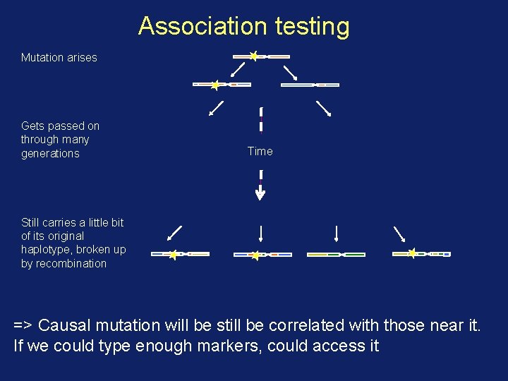
Association testing Mutation arises Gets passed on through many generations Time Still carries a little bit of its original haplotype, broken up by recombination => Causal mutation will be still be correlated with those near it. If we could type enough markers, could access it

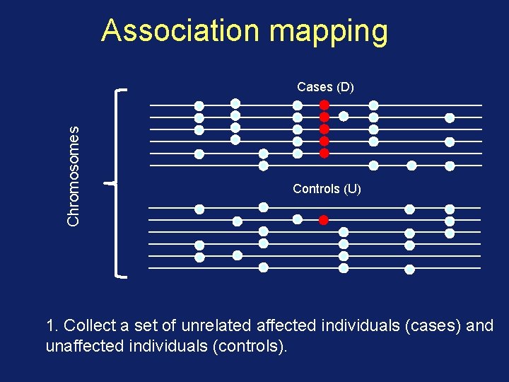
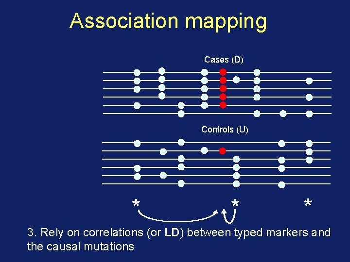
Association mapping Chromosomes Cases (D) Controls (U) 1. Collect a set of unrelated affected individuals (cases) and unaffected individuals (controls).

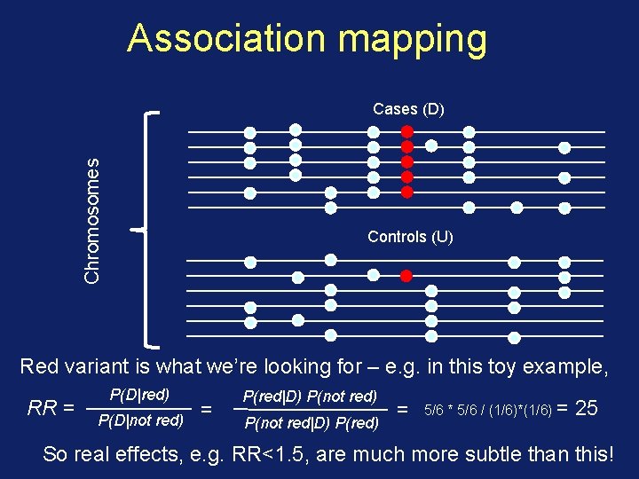
Association mapping Chromosomes Cases (D) Controls (U) Red variant is what we’re looking for – e. g. in this toy example, RR = P(D|red) P(D|not red) = P(red|D) P(not red|D) P(red) = 5/6 * 5/6 / (1/6)*(1/6) = 25 So real effects, e. g. RR<1. 5, are much more subtle than this!

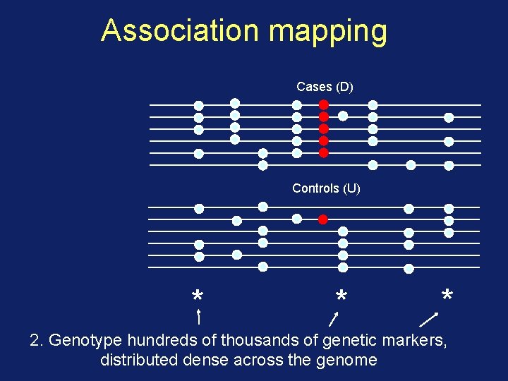
Association mapping Cases (D) Controls (U) * * * 2. Genotype hundreds of thousands of genetic markers, distributed dense across the genome

Association mapping Cases (D) Controls (U) * * * 3. Rely on correlations (or LD) between typed markers and the causal mutations

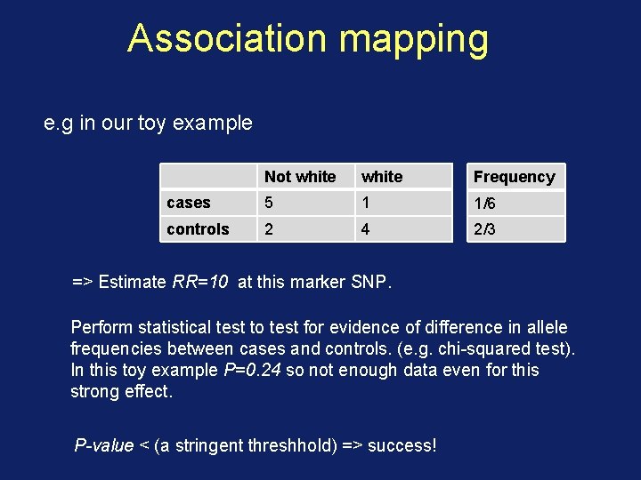
Association mapping e. g in our toy example Not white Frequency cases 5 1 1/6 controls 2 4 2/3 => Estimate RR=10 at this marker SNP. Perform statistical test to test for evidence of difference in allele frequencies between cases and controls. (e. g. chi-squared test). In this toy example P=0. 24 so not enough data even for this strong effect. P-value < (a stringent threshhold) => success!

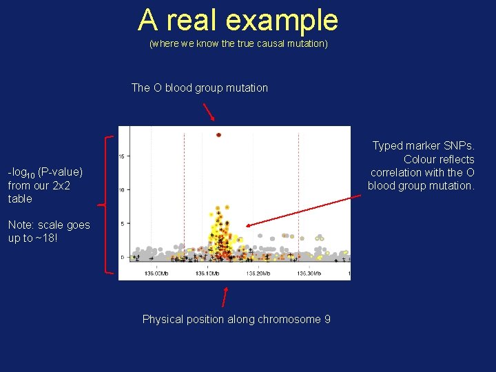
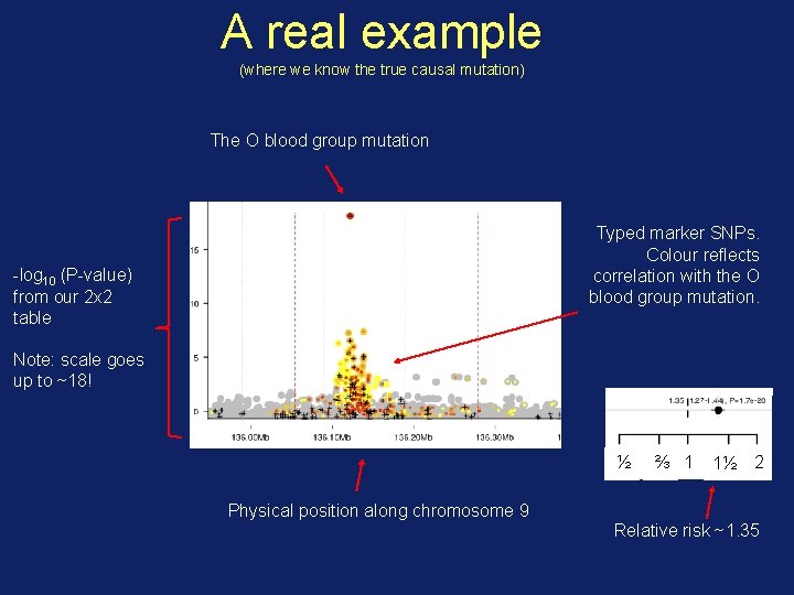
A real example (where we know the true causal mutation) The O blood group mutation Typed marker SNPs. Colour reflects correlation with the O blood group mutation. -log 10 (P-value) from our 2 x 2 table Note: scale goes up to ~18! Physical position along chromosome 9

A real example (where we know the true causal mutation) The O blood group mutation Typed marker SNPs. Colour reflects correlation with the O blood group mutation. -log 10 (P-value) from our 2 x 2 table Note: scale goes up to ~18! ½ Physical position along chromosome 9 ⅔ 1 1½ 2 Relative risk ~1. 35

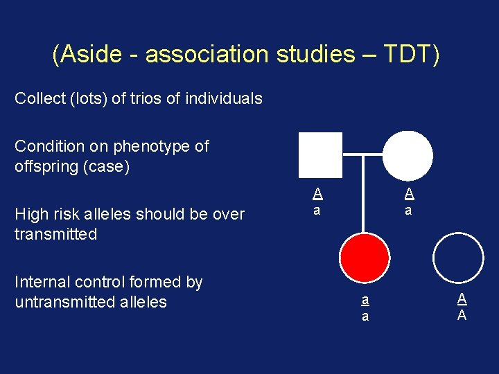
(Aside - association studies – TDT) Collect (lots) of trios of individuals Condition on phenotype of offspring (case) High risk alleles should be over transmitted Internal control formed by untransmitted alleles A a a a A A

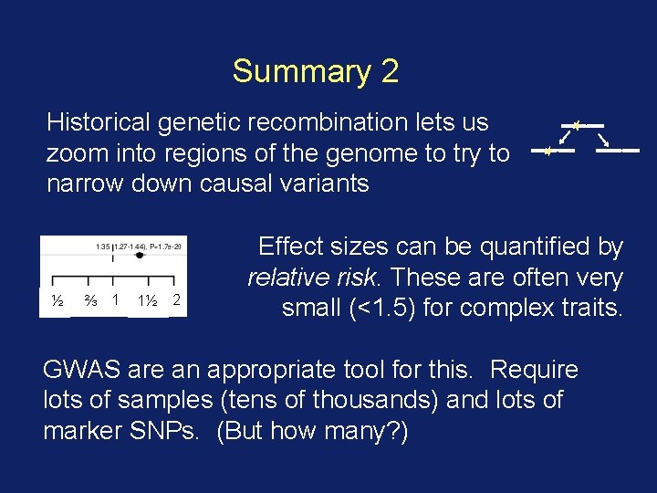
Summary 2 Historical genetic recombination lets us zoom into regions of the genome to try to narrow down causal variants ½ ⅔ 1 1½ 2 Effect sizes can be quantified by relative risk. These are often very small (<1. 5) for complex traits. GWAS are an appropriate tool for this. Require lots of samples (tens of thousands) and lots of marker SNPs. (But how many? )

The three pillars of GWAS Theory Association studies provide more power allowing us to detect the small effect sizes underlying gene responsible for common disease. Understanding human genetic diversity Understanding the structure of human genetic polymorphism and recombination Technology Can we actually type enough SNPs, and cheaply enough, for the large sample sizes required?

Understanding genetic diversity How many markers are actually required to tag the diversity? - To understand this, must first understand patterns of diversity in natural populations - Identify catalogue of variants to type Can we design experiments to analyse such large numbers of SNPs?

Genomics timeline Decade Technology #variants Discovery 1800 s 0 Pre-molecular genetics (Darwin; Mendel; Galton. . . ) 1900 s Handful Discovery of 1 st human polymorphism (the ABO blood group) 1950 s Structure of DNA published 1970 s “Sanger sequencing” Handful Low-throughout sequencing 1980 s RFLPs; PCR; 100 s First genetic marker linked to a disease (Cystic Fibrosis) found using a genetic linkage study. 1990 s Human Genome Project started. Linkage studies with 1, 000 s of markers. 2000’s Microarrays 105 -106 Human genome assembly completed; first surveys of human genetic variation (International Hap. Map project); first microarrays; first genome-wide association studies (GWAS). 2010’s highthroughput sequencing Whole genome Map of all common human variation (1000 Genomes Project); GWAS meta-analyses; direct-to-consumer genotype testing Today Very large scale ‘biobank’ / population sequencing projects.

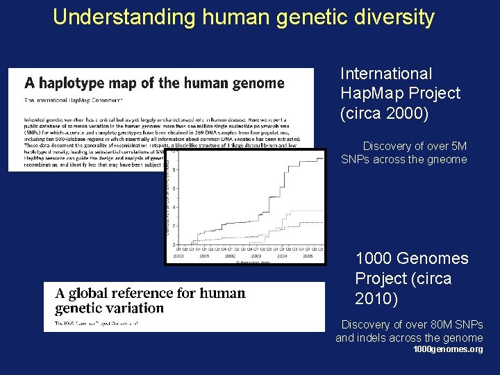
Understanding human genetic diversity International Hap. Map Project (circa 2000) Discovery of over 5 M SNPs across the gneome 1000 Genomes Project (circa 2010) Discovery of over 80 M SNPs and indels across the genome 1000 genomes. org

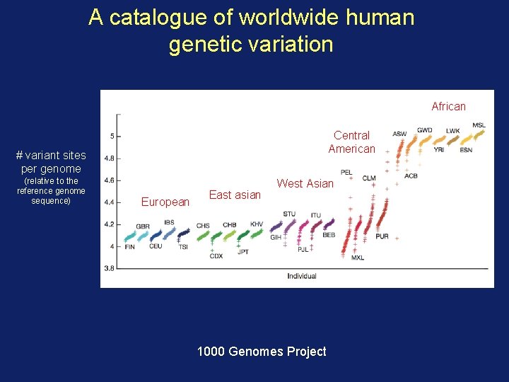
A catalogue of worldwide human genetic variation African Central American # variant sites per genome (relative to the reference genome sequence) European East asian West Asian 1000 Genomes Project

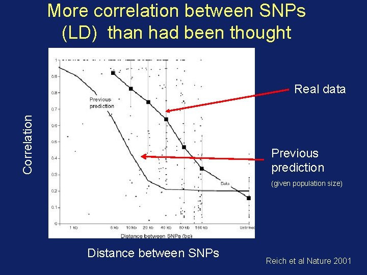
More correlation between SNPs (LD) than had been thought Correlation Real data Previous prediction (given population size) Distance between SNPs Reich et al Nature 2001

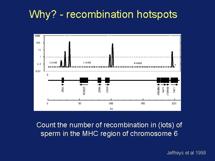
Why? - recombination hotspots Count the number of recombination in (lots) of sperm in the MHC region of chromosome 6 Jeffreys et al 1998

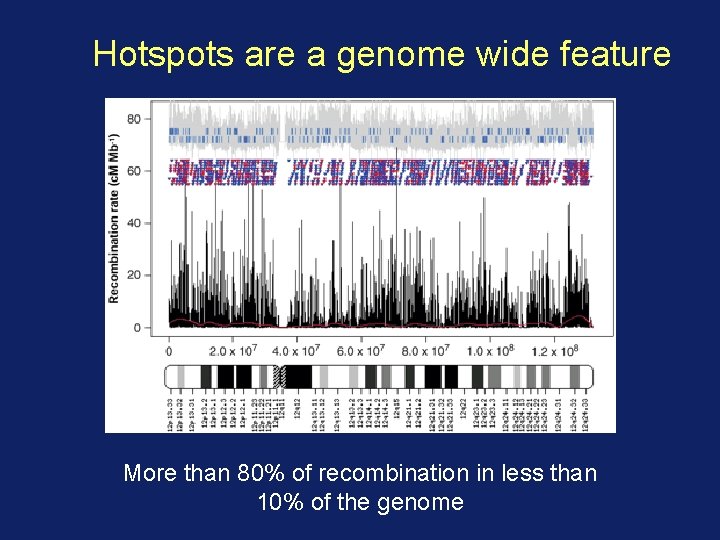
Hotspots are a genome wide feature More than 80% of recombination in less than 10% of the genome

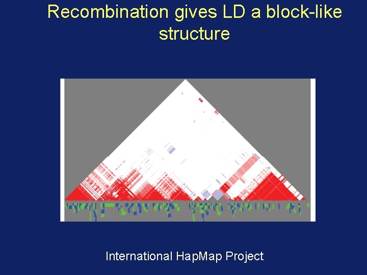
Recombination gives LD a block-like structure International Hap. Map Project

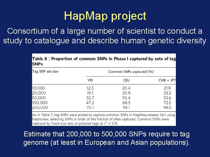
Hap. Map project Consortium of a large number of scientist to conduct a study to catalogue and describe human genetic diversity Estimate that 200, 000 to 500, 000 SNPs require to tag genome (at least in European and Asian populations).

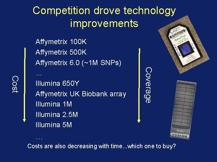
Competition drove technology improvements Coverage Cost Affymetrix 100 K Affymetrix 500 K Affymetrix 6. 0 (~1 M SNPs) … Illumina 650 Y Affymetrix UK Biobank array Illumina 1 M Illumina 2. 5 M Illumina 5 M … Costs are also decreasing with time. . . which one to buy?

Example The UK Biobank has typed ~500, 000 individuals on the Affymetrix UK Biobank array (containing ~800 k SNPs). This array might now cost ~£ 20 per sample. So this project would cost in the order of £ 10, 000 for genotyping.

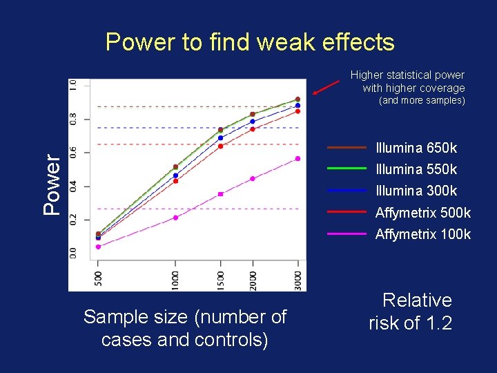
Power to find weak effects Higher statistical power with higher coverage (and more samples) Power Illumina 650 k Illumina 550 k Illumina 300 k Affymetrix 500 k Affymetrix 100 k Sample size (number of cases and controls) Relative risk of 1. 2

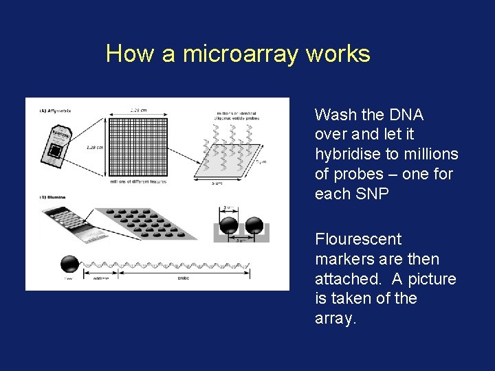
How a microarray works Wash the DNA over and let it hybridise to millions of probes – one for each SNP Flourescent markers are then attached. A picture is taken of the array.

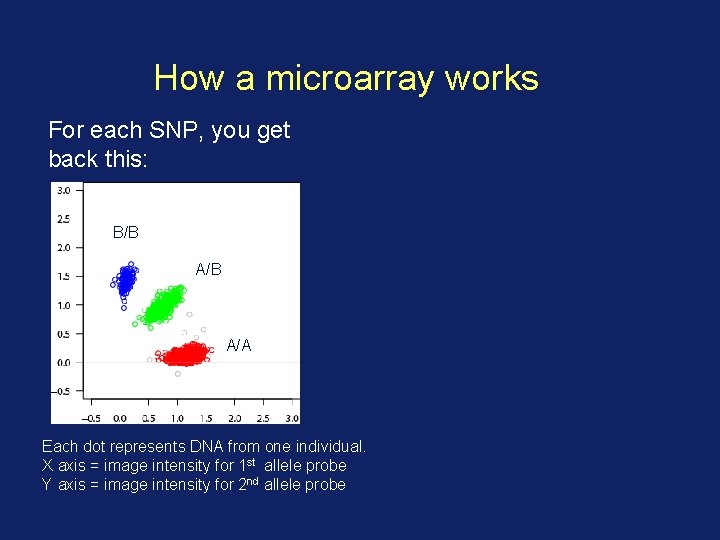
How a microarray works For each SNP, you get back this: B/B A/A Each dot represents DNA from one individual. X axis = image intensity for 1 st allele probe Y axis = image intensity for 2 nd allele probe

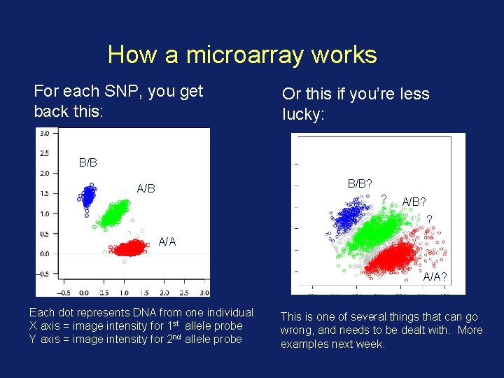
How a microarray works For each SNP, you get back this: Or this if you’re less lucky: B/B? A/B? ? A/A? Each dot represents DNA from one individual. X axis = image intensity for 1 st allele probe Y axis = image intensity for 2 nd allele probe This is one of several things that can go wrong, and needs to be dealt with. More examples next week.

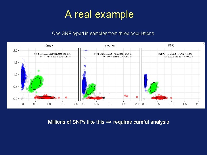
A real example One SNP typed in samples from three populations Millions of SNPs like this => requires careful analysis

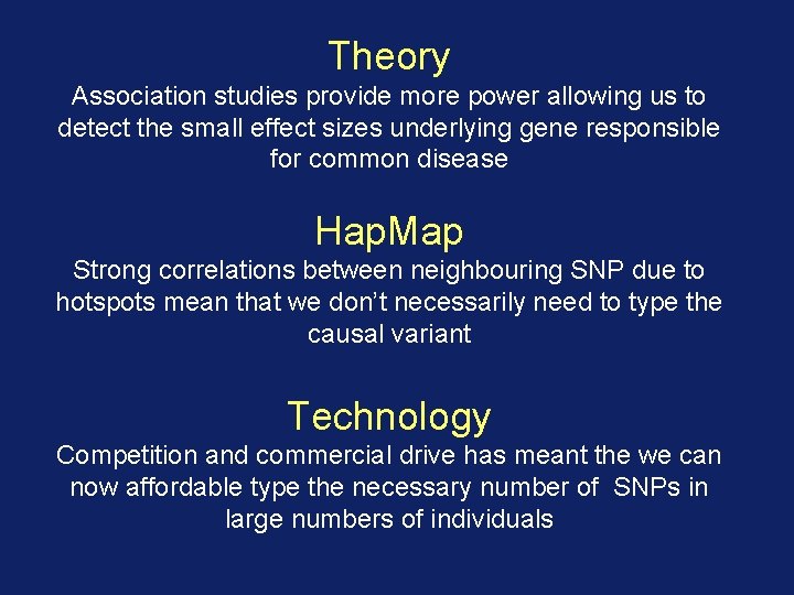
Theory Association studies provide more power allowing us to detect the small effect sizes underlying gene responsible for common disease Hap. Map Strong correlations between neighbouring SNP due to hotspots mean that we don’t necessarily need to type the causal variant Technology Competition and commercial drive has meant the we can now affordable type the necessary number of SNPs in large numbers of individuals

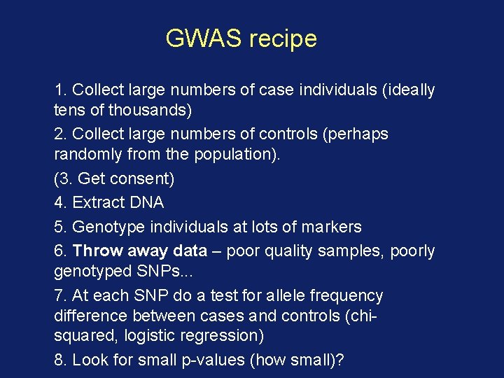
GWAS recipe 1. Collect large numbers of case individuals (ideally tens of thousands) 2. Collect large numbers of controls (perhaps randomly from the population). (3. Get consent) 4. Extract DNA 5. Genotype individuals at lots of markers 6. Throw away data – poor quality samples, poorly genotyped SNPs. . . 7. At each SNP do a test for allele frequency difference between cases and controls (chisquared, logistic regression) 8. Look for small p-values (how small)?

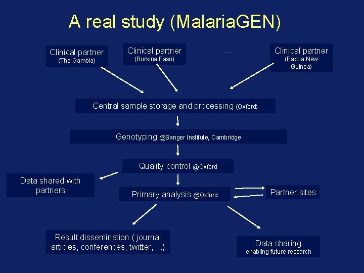
A real study (Malaria. GEN) Clinical partner (The Gambia) Clinical partner . . . Clinical partner (Burkina Faso) (Papua New Guinea) Central sample storage and processing (Oxford) Genotyping @Sanger Institute, Cambridge Quality control @Oxford Data shared with partners Primary analysis @Oxford Result dissemination ( journal articles, conferences, twitter, . . . ) Partner sites Data sharing enabling future research

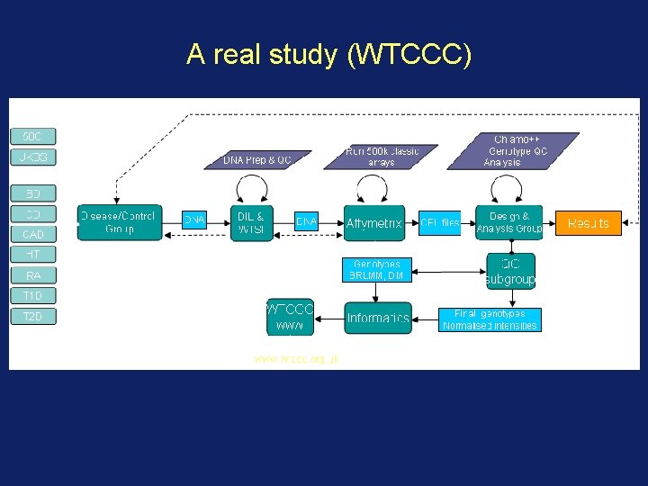
A real study (WTCCC)

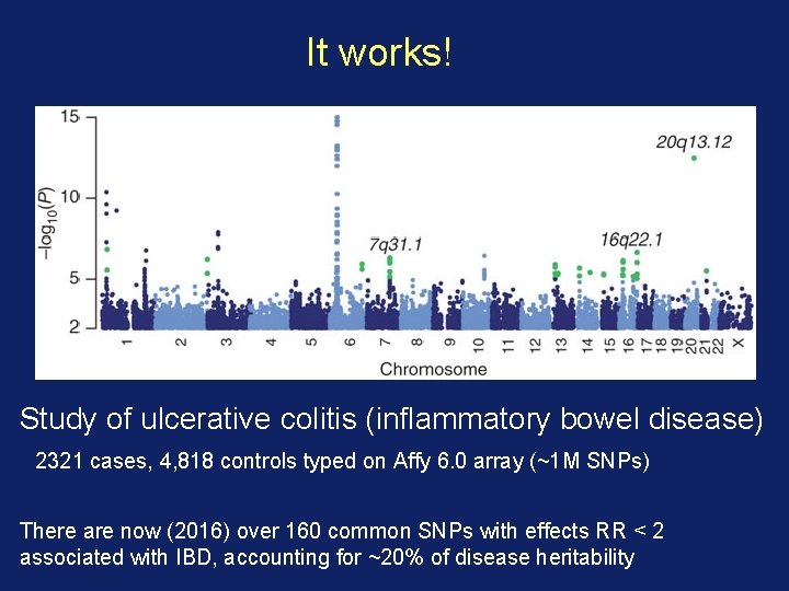
It works! Study of ulcerative colitis (inflammatory bowel disease) 2321 cases, 4, 818 controls typed on Affy 6. 0 array (~1 M SNPs) There are now (2016) over 160 common SNPs with effects RR < 2 associated with IBD, accounting for ~20% of disease heritability

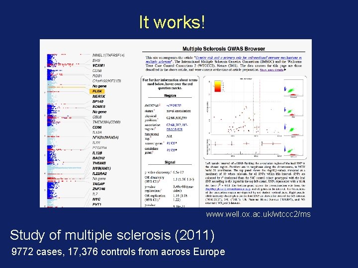
It works! www. well. ox. ac. uk/wtccc 2/ms Study of multiple sclerosis (2011) 9772 cases, 17, 376 controls from across Europe

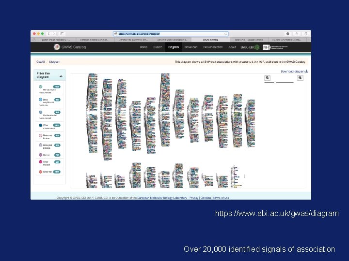
https: //www. ebi. ac. uk/gwas/diagram Over 20, 000 identified signals of association

Summary 3 It is clinically useful and interesting to look for the genetic variants contributing to human traits A combination of theory, understanding of population genetics, and technology has made it possible to carry out GWAS analysis. It works! But there are further challenges. . . Next week: look in detail at some real studies

Homework Visit http: //www. well. ox. ac. uk/wtccc 2/ms Play around with the site and make sure you understand the different things that are shown. Can you find the effect size (relative risk or ‘odds ratio’) for a variant? What frequency is the variant found at in the UK population? How does recombination affect the plots? What do the cluster plots tell you?