Multidisciplinary Design optimization incorporating Robust Design Approach to

Multidisciplinary Design optimization incorporating Robust Design Approach to tackle the uncertainties in the design of a Reusable Aerospace Vehicle Multidisciplinary Robust Design Optimization for a Reusable Aerospace Vehicle 1 st Progress Seminar after 6 months (Roll No. 02401701) Under the guidance of Prof. K. Sudhakar Prof. P. M. Mujumdar

FULLY REUSABLE TSTO TYPICAL FLIGHT PROFILE DEORBIT SATELLITE DEPLOYMENT RE-ENTRY DOWN/CROSS RANGE MANEUVERS RE-ENTRY SEPARATION AT 80 -100 KM, M 10 -12 PARACHUTE DEPLOYMENT LANDING MANEUVERS & LANDING ON AIR BAGS MANOEUVERS TURN HORIZONTAL LANDING CRUISE AT M 0. 8 & H=10 -12 KM SHYAM / LVDG

Expendable Launch Vehicle • Participating disciplines are. . Aerodynamics, Structures, Aero-thermodynamics, Navigation Guidance & Control, Propulsion and Mission & Trajectory. Reusable Launch Vehicle • Complexity = Launch vehicle + Space plane • Should also account for Life cycle Disciplines…. . Economics, Reliability, Manufacturability, Safety & Supportability • And should account for uncertainties

The Design Problem is… • Design of a reusable technology demonstrator for the First stage of Two Stage to Orbit fully reusable Launch Vehicle. For which the mission is defined as…

TYPICAL MISSION PROFILE OF RLV-TD ALT = 150 km RE-ENETRY / GLIDE / RANGE MANOEUVERS 2 G TURN ALT = 35 km S 12 SEPARATION ALT = 60 km M = 10. 0 FLYBACK CRUISE ALT = 12 km M=0. 8 LIFT-OFF LANDING

The Traditional Design Process Mission Requirements Configuration Concepts Historical Data base Engineering knowledge base Trade off based on Figures of Merit Historical Data base Concept Design & Vehicle Sizing Aerodynamics No Constraints met yes Eg: Space Shuttle, X-34, HYFLEX, ALFLEX, CRV Low fidelity Analysis Weight Propulsion Structures Estimation, CG Trajectory Analysis Stability & Control

Yes No Apply Small Perturbations in design variables Constraints met Low fidelity Analysis on Aero, Propulsion Weight Estimation & CG, Stability & Control and Trajectory Select the best No High fidelity analysis on Aerodynamics, Constraints met Structures, Weight & Cg estimation, Aerothermal Propulsion, Stability & Control and Trajectory yes Detailed Design

The methodology proposed in this research work Vehicle Conceptual Design using engineering methods (low fidelity) Aerodynamics, sizing, Propulsion, Stability& Control and Trajectory Design Noises variables factors Multidisciplinary Analysis (High fidelity) Sizing Optimiser Cost Model f, f Objective Functions Constraints INSCOST Aerodynamics CFD Propulsion Structure Empirical FEM Aerothermal MINIVER

The Configuration Concept selected

Parameterization of the vehicle configuration concept Airfoil 2 - for vertical tail

X 7 For wing

X 14

• X 1 to X 17 – Length parameters • t 1, t 2 – Thickness parameters • 1, 2 – Angular variables • R 1, R 2 – radii • di – internal diameter

• X 3 to X 8 and 1, 2 and the airfoil 1 are exclusively for the wing design. • Since accommodating the 24 variables for multidisciplinary robust design optimization, will be computationally expensive, the wing can be optimized separately for its intended performance and to take care of the variations due to operational & manufacturing uncertainties

The Constraints 1. The take off weight should not exceed 2000 Kg GTOW 2 T 2. The maximum diameter of the fuselage should be between 0. 9 to 1. 2 m 3. The volume requirement inside the fuselage for the avionics boxes, propulsion modules, landing gear wells and other auxiliary system are estimated as 3. 0 m 3 4. The nose cone length (x 1) is estimated as 2250 mm for the scramjet propulsion module performance point of view. x 1 = 2. 250 m 5. di, the internal diameter of the top half of the fuselage = 1. 00 m (considering the interfacing requirement with the solid boosters of 1 m diameter)

6. The bottom surface of the demonstrator should be flat so that the scramjet modules integration as well as the inlet conditions are satisfied. Also for easy mounting of the Thermal Protection System tiles. This will compel the selection of an airfoil with flat bottom for the wings. 7. 8. The hypersonic L/D 1. 5 Subsonic L/D max = 4. 5 9. The landing weight of the vehicle also should be taken as 2. 00 T to take care of abort scenario. 10. For subsonic cruise, Lift L = 2000 kg, for Mach 0. 8 at 12 km altitude 11. Wing leading edge sweep 45 and leading edge radius should be for minimum re-entry heating. 12. For the subsonic cruise, the drag (D) of the vehicle should be equal to the thrust deliverable

14. The cruise range 800 km. 15. The touch down speed 80 m/sec and the landing angle of attack will be 15 deg. 16. The sink rate at touch down 4. 5 m/sec. 17. The runway roll 1. 8 km. 18. During the ascend boost phase the maximum dynamic pressure should be 120 KPa and angle of attack should be less than 3 degree and Maximum longitudinal acceleration should be 10 g 19. During the re-entry phase the dynamic pressure should be less than 20 KPa and the maximum lateral acceleration should be 3 g 20. During re-entry the overall heat flux should be less than 50 Watts/sq-cm

The objective function Maximize the cruise range Uncertainties Expected Manufacturing Uncertainty – which will result in surface roughness and the excrescence effects, like mismatches , gaps, contour deviation and fastners flushness (rivets, etc) on the wetted surface. Operational Uncertainty – like uncertainty in cruise Mach number.

Literature Survey Parametric Optimization of Manufacturing Tolerances at the aircraft surface - A. K. Kundu, John Watterson, and S. Raghunathan, Journal of Aircraft, Vol. 39, No. 2, March-April 2002. Ø Aimed at reducing life cycle cost of the passenger aircraft by relaxing the manufacturing tolerances on 11 key features in the nacelle. ØParasite drag increase resulted by the degradation of the surface smoothness qualities, for example, the discrete roughness on the component parts and at their subassembly joints. These are seen as aerodynamic defects, collectively termed as one of the excrescence effects, typically, i) mismatches (steps etc. ) ii) gaps, iii) contour deviation and iv) fastners flushness (rivets, etc) on the wetted surface.

The four types of surface excrescence at the key manufacturing features
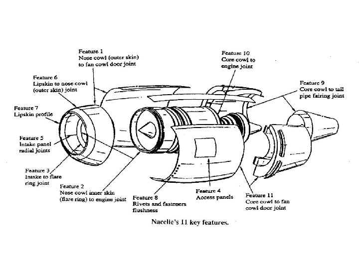
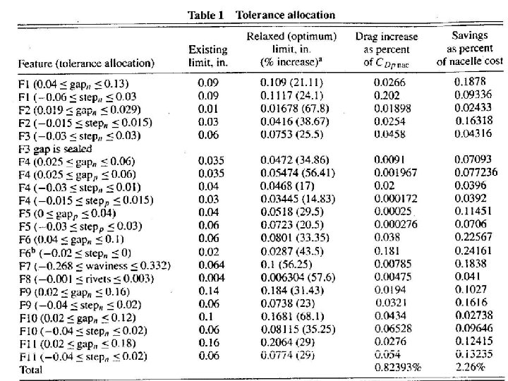

Findings Ø The results show that feature by feature percentage changes for one nacelle with a drag coefficient increment of 0. 824% and a reduction of 2. 26% on the nacelle cost. Ø This will result to 0. 421% overall reduction in DOC (Direct Operating Cost) of the transport aircraft. Ø Tolerance relaxation tradeoff study between drag increase (loss of quality function) and manufacturing cost reduction (gain). Ø Further research work is planned by the same group to extend the study to wing and fuselage.

Probabilistic Approach to Free-Form Airfoil Shape Optimization Under Uncertainty - Luc Huyse, AIAA Journal, Vol. 40, No. 9 September, 2002 Luc Huyse, R. Michael Lewis, “Aerodynamic Shape Optimization of Twodimensional Airfoil Under Uncertain Conditions” [16], NASA/CR-2001210648 q This work is on the operating uncertainties which will affect the performance of an aircraft. The airfoil shape optimization is addressed. q In airfoil design, the objective is to minimize drag with the specified cruise Mach number and target lift coefficient q Robust design of airfoils for a transport aircraft. Here robust design technique accounts for the variation in cruise Mach number.

The objective is lift constrained wave drag minimization over the Mach range M [0. 7, 0. 8]: min Cd (d, M) d D Sub to Cl (d, M) Cl* over M [0. 7, 0. 8] Where d is the vector of design variables and D is the design space. Cl* is the minimum lift corresponds to typical values found for commercial transport airliners. In this study, the Mach number is the only uncertain parameter. This deterministic optimization model is not necessarily an accurate reflection of the reality. The formulation contains no information regarding off-design condition performance. So the drag reduction is achieved only over a narrow range of Mach numbers. This is of concern if substantial variability is associated with operating condition.

Consider different Mach numbers and to generalize the objective function to a linear combination of flight conditions: m min Wi Cd (d, Mi) d D i=1 Sub to Cl (d, Mj) Cl* For j = 1, 2, …. . m Practical problems arise with the selection of flight conditions (Mi) and with the specification of the weights Wi. There are no clear theoretical principles to guide the selection, which is in fact, largely left to the designer’s discretion. With multipoint formulation, Cd can be realized over a wide range of Mach numbers M, however this formulation is still unable to capture the full range of uncertainty.

Nondeterministic Approach M is now treated as a random variable and the optimization problem is now interpreted as a statistical decision making problem. So using the probability density function of the Mach number, the objective function is stated as min Cd (d, M) f. M(M) d. M Sub to Cl (d, Mj) Cl* for all M, where f. M(M) is the probability density function of the free flow Mach number M. The practical problem is that integration is required in each of the optimization steps. Theoretically sound but computationally expensive. This work is an example of using probabilistic approach in achieving robustness, provided the distribution pattern of the noise variable is known.

* Robert H. Sues, Mark A. Cesare, Stephan S. Pageau, & Justin Y. -T. Wu, “Reliability – Based Optimization Considering Manufacturing and Operational Uncertainties”[13], Journal of Aerospace Engineering, October, 2001 Discuss about the approach of integrating MDO and probabilistic methods to perform reliability based MDO. RBMDO Demonstrated on – Passenger Airplane Wing Design problem • Objective : Maximize expected cruise range • Subjected to constraints • 1. P (upper surface root stress 1 ≤ y ) ≥ 99. 0 % • • -6. P (take off distance ≤ 3000 ft ) ≥ 99. 0 %

3 case studied Case A: Six deterministic constraints with no safety factor on yield stress Case B : Six deterministic constraints with safety factor of 1. 5 on yield stress Case C: Six probabilistic constraints • Manufacturing uncertainties are simulated on design variables • Operational uncertainties are considered. The results show that: RBMDO ( case C ) gives optimum solution that balances performance and reliability Range : (NM) Reliability: (%) Case A Case B Case C 1024. 7 984. 7 974. 9 38 96 99

* P. B. S. Reddy and K. Nishina, Dr. Subash Babu “Taguchi’s methodology for multi-response optimization- A case study in the Indian plastic industry”[6]- International journal of Quality & Reliability Management, Vol. 15, No. 6, 1998, pp. 646 -668 • Taguchi’s methodology for carrying out a robust design is narrated in this. • The salient features of robust design are presented and the robust design methodology applied to the case having multi responses (for an injection moulding process for the agitator of washing machine) is presented. • The output responses considered were outer diameter, height & pull out force.

• The goal was minimizing the variance of the height, and outer diameter of the agitator while keeping the mean on target and pull out strength <1. 8 kg/sq-cm • Based on cause-effect diagram seven factors were identified • Three noise factors identified were - change of machine operators, variation in raw material quality and change in temperature & environmental conditions. • By performing robust design in the specific case of injection moulding process the rejection rate could be reduced from 20 % to zero percent which helped the company in many ways related to cost, delivery, quality & productivity.

* K. K. Choi, B. D. Youn, “Issues Regarding Design Optimization Under Uncertainty”, http: //design 1. mae. ufl. edu/~nkim/indexfiles/choi 4. pdf Discusses the mathematical formulation of robust design problems The conventional optimization model is defined as Minimize OBJ (d) Sub. to Gi (d) 0, i = 1, 2, …. NC d. L d d. U where OBJ is the objective function, Gi is the ith constraint function, NC is the number of constraints, d is the design variable vector, d. L & d. U are the lower & upper bounds of d.
![In robust design, Minimize OBJ [ R, R ] sub. to Gi ( )](http://slidetodoc.com/presentation_image_h/9b61a805879ab1f281be73b0c36f47e0/image-33.jpg "In robust design, Minimize OBJ [ R, R ] sub. to Gi ( )")
In robust design, Minimize OBJ [ R, R ] sub. to Gi ( ) + k Gi 0 , i = 1, 2, …. NC d. L d d. U where R, R are the mean & standard deviation of the response R, Gi ( ) and Gi are the mean & standard deviation respectively of the ith constraint function, k is the penalty function decided by the designer, d is the design variable vector, d. L & d. U are the lower & upper bounds of d.
![NPR OBJ [ R, R ] = [ w 1 j ( Rj –](http://slidetodoc.com/presentation_image_h/9b61a805879ab1f281be73b0c36f47e0/image-34.jpg "NPR OBJ [ R, R ] = [ w 1 j ( Rj –")
NPR OBJ [ R, R ] = [ w 1 j ( Rj – Rj t ) 2 + w 2 j 2 Rj ] J=1 sub. to Gi ( ) + k Gi 0 , i = 1, 2, …. NC d. L d d. U Where, w 1 j is the weight parameter for mean on target, w 2 j that for the jth performance to be robust, Rj and Rj the mean and standard deviation of the jth performance, Rj t is the target value of the jth performance and NPR is the number of performances to be robust.

For the robust design for best overall performance over the entire life time the objective function is based on the joint probability density function of the random variable x. NPR OBJ ( d, x ) = x wj Rj (d, x) f x (x) dx J=1 s. t Gi ( ) + k Gi 0 , i = 1, 2, …. NC d. L d d. U Where f x (x) is the joint probability density function of the random variable x, Rj (d, x) is the jth performance function to be minimized and wj is the weight parameter for the jth performance to be robust.
 problem Minimize OBJ (d) s. t P")
Mathematical formulation of reliability based design (RBDO) problem Minimize OBJ (d) s. t P { ( Gi (d ) c } CFLi , i = 1, 2, …. NC d. L d d. U where CFLi is the confidence level associated with the ith constraint, P denotes the probability, Gi (d ) is the ith constraint function and c is the limiting value. Example: P ( stress 1 y ) 99. 0 % , where y is the yield stress. (ie) Since there are some uncertainty in the material properties, instead of stating the constraint as, stress 1 y, it is stated as the probability of stress 1 y, is greater than or equal to 99. 0%.

Robust & Reliability Based Design. When the objective function is based on the robust design principle, focusing on making the response insensitive to the variations in the design variables and the constraints are modified to probabilistic constraints with the assigned probability of each constraint function, the result is a Robust & Reliability Based Design (RRBDO) The mathematical formulation of such a method is given below. Minimize OBJ [ R, R ] s. t P { ( Gi (d ) c } CFLi , i = 1, 2, …. NC d. L d d. U where NC is the number of constraints and the objective function is defined as NPR OBJ [ R, R ] = [ w 1 j ( Rj – Rj t ) 2 + w 2 j 2 Rj ] J=1

Plan of Action for the Next Two Years Robust & Reliability Final based MDO of thesis Integration of MDO Aerospace vehicle submission architecture with design robust design techniques & Draft thesis probability analysis preparation, review & modifications Understanding, practising & applying stochastic techniques Exploring the options for probabilistic design & applying to the problem Activity Identifying & understanding the uncertainty analysis methods Identifying a proper strategy to attack the problem Review of the strategy & modifications Defining the design problem, identifying the constraints, control variables, noise factors & objective functions. 2 nd Progress seminar Literature Survey & exploring in-depth information on robust & reliability based design practices, techniques & the related research works around the globe August, 03 Month / Year August, 04 August, 05

Acknowledgement I would like to express my sincere thanks to Prof. K. Sudhakar and Prof. P. M. Mujumdar of Aerospace Engineering Department for their continuous guidance, encouragement and support.


Methods of simulating the variation in noise factors • Monte Carlo Simulation • Taylor Series Expansion • Orthogonal Array based Simulation • Monte Carlo Simulation A random number generator is used to simulate a large number of combinations of the noise factors called testing conditions. The value of the response is computed for each testing conditions and the mean and variance of the response are then calculated. For obtaining accurate estimate of mean & variance, the Monte Carlo method requires evaluation of the response under a large number of testing conditions. This can be very expensive, especially if we also want to compare many combinations of

Methods of simulating the variation in noise factorscont’d • Taylor Series Expansion The mean response is estimated by setting each noise factor equal to its nominal value. To estimate the variance of the response, the derivatives of the response with respect to each noise factor is found out. Let R denote the response and 12 , 22, ……… n 2 denote the variance of n noise factors. The variance of R is then computed by the formula: R 2 n = ( R / xi)2 i 2 , i=1 where x. I is the ith noise factor.

Methods of simulating the variation in noise factorscont’d • Orthogonal Array based Simulation Orthogonal arrays are used to sample the domain of noise factors. For each noise variable different levels are taken. The advantage of this method over the Monte Carlo method is that it needs a much smaller number of testing conditions; yet the accuracy will be excellent. The orthogonal array based simulation gives common testing conditions for comparing two or more combinations of control factor settings.

* Amy E. Kumpel, Peter A. Barros Jr. , and Dimitri N. Mavris “Quality Engineering Approach to the determination of the Space Launch capability of the peace keeper ICBM utilizing probabilistic methods” [1] - AIAA 2002 -10 -6 Discuss about the use of a comprehensive and robust methodology for the conceptual design of an expendable launch vehicle employing the existing Peacekeeper ICBM This methodology includes an Integrated Product and Process Development (IPPD) approach, coupled with response surface techniques and probabilistic assessments. It also provides a probabilistic framework to address the inherent uncertainty in vehicle requirements in an analytical manner by representing payload, mission, and design requirements as distributions instead of point values. The three primary objectives identified are (i) to design for the minimization of the time-to-launch, (ii) minimization of development and production costs, and (iii) the maximization of useable payload

The first step in the design process was to define the problem by mapping the customer requirements to engineering characteristics. A Quality Function Deployment approach, utilizing a House of Quality, was employed. Possible engine and propellant types, as well as staging arrangements, were organized in a Morphological Matrix of design alternatives. Several vehicle concepts from the Morphological Matrix were then evaluated in terms of performance, cost, availability, reliability, safety, commonality with existing space systems, and compatibility with various launch sites. Ranges were assigned to several significant design variables, and a sensitivity analysis was performed on the responses to see how small perturbations in the design variables would affect the outcome. A parametric study was also performed on some of the assumptions made in the design process so that the exact effects of the estimates on the vehicle concept could be determined. A Response Surface Methodology (RSM) in conjunction with a Monte Carlo simulation was used for these tasks. This methodology was an iterative process and was repeated until both technical feasibility and economic viability were achieved.

The tool employed in the problem definition stage of this study was the Quality Function Deployment (QFD) process which is a "planning and problem solving tool that is finding growing acceptance for translating customer requirements into the engineering characteristics of a product”. The broad requirements of the engineering characteristics are transformed into an interrelationship digraph (ID). A statistical analysis software package called JMP is used to create the Do. Es. A Monte Carlo simulation is used in conjunction with response surface equations in order to model thousands of designs in seconds. The software package Crystal Ball by Decisioneering® is used for this task. Crystal Ball is a risk analysis software package and an add-in to Microsoft Excel. It allows for the definition of design variables as probability functions bounded by a range or a set of values. It then uses the defined ranges in a Monte Carlo simulation. For each uncertain design variable, a probability distribution is used to define the possible values. Distribution types include normal, triangular, uniform, logarithmic, etc. The Monte Carlo simulation creates Probability Distribution Functions (PDFs) and Cumulative Distribution Functions (CDFs), in order to illustrate the probability of success for a response.

A PDF is the mathematical function that maps the frequency of the response to metrics within the given range. The PDF is then integrated to determine a CDF. The CDF is the mathematical function that maps the probability of obtaining a response to the metric within the given range. If the amount of feasible design space is unacceptable, three options exist for the designer/decisionmaker: 1. Modify the design variable ranges; 2. Relax the constraints; 3. Select a different alternative concept. At this point in the design process, the system is evaluated to check if the responses satisfy the customer requirements as established in the problem definition phase. If any of the requirements are violated at any point in this iterative process, the design process will be repeated.

* Brent A. Cullimore , “Reliability Engineering & Robust Design : New Methods for Thermal / Fluid Engineering”[14], C & R White Paper, Revision 2, May 15, 2000 Mention that overdesign provides robustness but it is costly in areas such as aerospace. He modified SINDA/FLUINT, thermodynamic analyzer software to make the design robust by statistically integrating the probabilities of design variables to control the probability of response. The paper dwells on the SINDA/FLUINT software and also mention about the add on software named Relaibility Engineering module, which will estimate the reliability of a point design based on uncertainties in the dimensions, properties, boundary conditions etc.
 A design can")
Few possible capabilities of Reliability Engineering Module in SINDA/FLUINT (1) A design can be selected using the solver and then (in the same or later run) the reliability of that design can be estimated. (2) The reliability of a design can be used as an objective (maximize reliability or minimize the chances of failure). (This feature can be useful to the present problem). (3) The reliability of a design can be used as an optimization constraint (find the minimum mass design that achieves a reliability of at least 99%). (4) The range or variance of a random variable can be used as a design variable What variations can be tolerated : how tight must tolerance be ? . The paper also mention about a commercial tools named Engineous i. SIGHT ® that can perform optimization, reliability estimation and robust design generation.

* Wei Chen, Kemper Lewis, “A Robust Design Approach for Achieving Flexibility in Multidisciplinary Design”[2], http: /www. uic. edu/labs/ideal/pdf/Chen. Lewis. pdf (2001) Explained the two types of robust design. In type 1, the robust design concept is applied to the early stages of design for making decisions that are robust to the changes of downstream design considerations (called Type I robust design). Furthermore, the robust design concept is extended to make decisions that are flexible to be allowed to vary within a range (called Type II robust design) [2, 18]. In Type II robust design, the performance variations are contributed by the deviations of control factors (decision variables) rather than the noise factors. The concept behind Type II robust design for determining flexible design solutions is represented in Figure below.

For a typical optimization model that is stated below The robust optimization can be formulated as a multiobjective optimization problem shown as the following:

f and f are the mean and the standard deviation of the objective function f (x), respectively. In the above equation, the mean locations and the range of design solutions are identified as x and ? x. To study the variation of constraints, the worst case scenario is used, which assumes that all variations of system performance may occur simultaneously in the worst possible combination of design variables. To ensure the feasibility of the constraints under the deviations of the design variables, the original constraints are modified by adding the penalty term to each of them, where kj are penalty factors to be determined by the designer. The bounds of design variables are also modified to ensure the feasibility under deviations. Depending on the computation resource, f and f could be obtained through simulations or analytical means such as Taylor expansions.

Improving the quality of a product through minimizing the effect of the causes of variation without eliminating the causes To assure proper levels of safety (Probability of being safe) for the system designed

* Wei Chen, Xiaoping Du, “Efficient Robustness and Reliability Assessment in Engineering Design”, www. icase. edu/colloq/data/colloq. Chen. Wei 2001. 5. 9. html (2001) Narrates the difference between Robust Design & Reliability based Design and Integrated Robust & Reliability Assessments and schematically presented the procedure for optimization under uncertainty. Uncertainty Classification Impact of events Catastrophe Risk analysis Reliability based Design & optimization Performance loss Cost benefit analysis Robust Design & optimization Everyday fluctuations Extreme events Frequency of events

And the difference in problem formulation for Conventional Optimization model & Robust Design model is given as below. Integrated Robustness & Reliability Assessments

* Stephen M. Batill, John E. Renaud, Xiaoyu Gu “Modeling & Simulation Uncertainty in Multidisciplinary Design Optimization” – AIAA-2000 -4803 Dwell on the technical risk & uncertainty in the model based design of physical artifacts. The issues of physical process variability, information uncertainty and the influence of the use of models & simulations on the design decision process are discussed. This paper only qualitatively addresses these issues. It suggests Monte Carlo simulation for uncertainty analysis in which variations in the design variables & parameters are selected from an appropriately selected population of random numbers.
![* Daniel P. Schrage “Technology for rotorcraft affordability through Integrated Product/Process Development (IPPD)” [19]–](http://slidetodoc.com/presentation_image_h/9b61a805879ab1f281be73b0c36f47e0/image-57.jpg "* Daniel P. Schrage “Technology for rotorcraft affordability through Integrated Product/Process Development (IPPD)” [19]–")
* Daniel P. Schrage “Technology for rotorcraft affordability through Integrated Product/Process Development (IPPD)” [19]– 55 th Annual Forum of American helicopter Society, May 25 th – 29 th, 1999. Highlights the Robust Design Simulation as the main approach in the roadmap to Affordability. He defines the benefit -cost ratio (BCR) as an objective and defines robust design as the systematic approach to find optimum values of design factors which results in economical designs which maximize the probability of success. The steps in economic risk analysis & other research activities in the related areas at Georgia Tech are mentioned.

Focus on to the specific Aerospace Vehicle Design Problem • To design a reusable technology demonstrator ( for the First stage of Two Stage to Orbit fully reusable Launch Vehicle. ) TSTO Features • 10 T to LEO (Low earth Orbit) payload capability • Vertical take off • Semicryogenic booster stage with Isp of 330 sec (mission average) & cryogenic orbiter stage Isp 400 sec (mission average) • Total lift off weight < 700 tons • Winged body booster which should boost the orbiter to Mach 10 at altitude of 80 -100 km then separate, return to launch site land horizontally in a conventional runway of 2. 5 km stretch.

• The vehicle structures should be designed for 100 flights & engine/ stage systems should be for 50 flights • Turn around time should be 30 days • The service life of the vehicle should be 15 years • Ideal velocity at 400 km circular orbit =9. 8 km/sec • Number of missions < Ten per year • Payload fraction = 2% (Measure of efficiency of the vehicle) • Cost effectiveness < $1000/kg for the LEO payload • Realizability – Total development time <10 years • Reliability >0. 995 (Other features which are not relevant to the specific design problem are not mentioned) • The mission profile of the TSTO vehicle is shown in the next slide.

Flying regimes and related parameters of the TSTO first stage • Vertical lift off with T/W of 1. 3 (GLOW < 700 tons) • Maximum acceleration (longitudinal) during ascend phase < 10 g • During the ascend boost phase the maximum dynamic pressure should be 120 KPa and angle of attack should be less than 3 degree • Separation altitude & velocity =80 -100 km & Mach 10 • Re-entry altitude = 100 -80 Km • Angle of attack during re-entry 40 deg • During the re-entry phase the dynamic pressure should be less than 20 KPa and the maximum lateral acceleration should be 3 g • Maximum Heat flux during re-entry < 50 Watts /sq-cm • Turn around manoeuvres by aero control surfaces – Elevons & rudders

• • Cruise Mach number =0. 8 Cruise altitude = 12 km Down range at cruise start = 800 km Angle of attack at touchdown < 15 deg Horizontal velocity at touch down = 80 -100 m/sec The sink rate at touch down < 4. 5 m/sec The landing roll shall be < 2 km So the task is to design a Technology demonstrator for the first stage of this TSTO
 is 85 m/sec 2. Subsonic L/D max")
Design Guidelines 1. Maximum landing speed (horizontal) is 85 m/sec 2. Subsonic L/D max = 4. 5. 3. The vehicle should have near neutral stability at subsonic speeds. 4. The vehicle should be trimmable at all Mach numbers. 5. The vehicle takes off vertically and lands horizontally hence the wing design should be for landing and checked for the other flight regimes. 6. It should have minimum pitching about CG for mated configuration, with the solid boosters. 7. The hypersonic L/D shall be 1. 5 for better cross range. – cont’d

8. The landing weight of the vehicle is taken as equal to the take off weight to take care of the abort missions. 9. The wing loading should be selected in such a way that the structural weight is minimum. 10. Wing plan form should be selected for the best performance in hypersonic as well as subsonic regimes. 11. Wing should provide a lift equal to the GTOW during cruise at subsonic speed (Mach 0. 8) at altitude of 12 km. 12. The airfoil should be selected to have maximum Cl at landing and lower heating at hypersonic speed as well as for mounting of tiles, the bottom flat airfoil is preferred. 13. The control surfaces should be sized to trim the vehicle with minimum force and maintain the attitude at hypersonic speed. – cont’d

14. Fuselage fore body should be shaped so as to minimize the re-entry heating, to have minimum drag and for good directional stability. 15. Wing leading edge sweep shall be not less than 45 deg. 16. Wing leading edges shall be blunted to reduce re-entry heating. 17. Low aspect ratio wing with highly swept leading edge angle shall be considered to reduce heating and drag. 18. Thickness of airfoil shall be selected based on lift, drag & leading edge bluntness requirements. 19. Vertical tail area should be designed to provide positive directional stability and rudder shall be designed for landing conditions at high angle of attack in cross-wind aft C. G conditions. – cont’d

20. The gaps between control surfaces and aerosurfaces shall be kept minimum to reduce the heating problems & to improve the performance. 21. The fuselage should be sized considering the volume requirements for accommodating the avionics systems, propulsion modules, landing gears and other auxiliary systems and also for better interfacing with the carrier solid boosters. 22. The vehicle should be capable of testing the scramjet module in a dedicated mission. 23. The vehicle should have a supersonic cruise capability at Mach 3. 0 using the ramjet engine.

After analysing the additional requirements in terms of technology, from all the entities the major objectives of the RLV-TD are listed as follows [23]. • (i) To evaluate the aero-thermo dynamic characteristics of wing body vehicle and associated control surface effectiveness at various flight regimes i. e. from sub-sonic to hypersonic zones. • (ii) schemes to function in the demanding environment of re-entry, cruise flight and auto-landing phase with constraints on loads and thermal environment. • (iii) To demonstrate the auto-landing technologies including landing gear, aerodynamic control, deceleration systems etc. valuate To • (iv) weight structures for multiple missions (say about 100), evaluation of air-breathing propulsion system, to design and validate redundant electro-mechanical actuators to control the vehicle at severe environment condition. • (v) operation requirements. • (vi) To demonstrate the scramjet propulsion module.

The Challenges • The multidisciplinary nature • The coupling with different disciplines and a large design variable set • Uncertainties of parameters and model structure • The computational burden The best solution to tackle the uncertainties is the robust design solution (ie) by making a design insensitive to the variations in noise factors and to tackle the variation in the control factors a reliability based solution in which the constraints are stated probabilistically to get the probability of an objective function for a known deviations in the control factors.

Information flow of a Multidisciplinary System

Complex ities of MDO under Uncertainties Xs- the sharing variables Xi-the design variables of subsystem (discipline) i, Yij-linking variables of subsystem Zi-output of subsystem i

A Typical model with uncertainties

The major disciplines involved in the design of the aerospace vehicle are Aerodynamics, Structures, Aero-thermodynamics Propulsion and control. (1) Aerodynamics F 1 (Xs, X 1, Y 21 ----Y 51) (2) Structures F 2 (Xs, X 2, Y 12 --Y 52) (3) Propulsion F 3 (Xs, X 3, Y 13 --Y 53) 3 (Xs, X 3, Y 13 --Y 43) RMDO (4) Control F 4 (Xs, X 4, Y 14 --Y 54) 4 (Xs, X 4, Y 14—Y 54) (5) Aero-thermodynamics F 5 (Xs, X 5, Y 21 ----Y 51)

* K. K. Choi, B. D. Youn, “Issues Regarding Design Optimization Under Uncertainty”, http: //design 1. mae. ufl. edu/~nkim/index-files/choi 4. pdf Emphasizes the different ways of applying the term robustness as, Definition 1 - Identify designs, which minimize the variability of the performance under uncertain (manufacturing or operation) conditions, Definition 2 -Provide the best overall performance over the entire lifetime of the structure or device and Definition 3 - Mitigate the detrimental effects of the worst-case performance. The design with the “best” worst-case performance is selected as the robust solution as per definition 3. The conventional optimization model is defined as Minimize OBJ (d) s. t Gi (d) 0, i = 1, 2, …. NC d. L d d. U where OBJ is the objective function, Gi is the ith constraint function, NC is the number of constraints, d is the design variable vector, d. L & d. U are the lower & upper bounds of d.

In robust design, of definition 1 the objective is to keep the mean on target & minimize the variation. So the mean & standard deviation of the response will constitute the objective function. So the formulation will be Minimize OBJ [ R, R ] s. t Gi ( ) + k Gi 0 , i = 1, 2, …. NC d. L d d. U where R, R are the mean & standard deviation of the response R, Gi ( ) and Gi are the mean & standard deviation respectively of the ith constraint function, k is the penalty function decided by the designer [5], d is the design variable vector, d. L & d. U are the lower & upper bounds of d. Here the objective function takes care of the signal & noise factors and the constrained functions are modified such that the allowed variation in them are limited by the sigma bounds.
![NPR OBJ [ R, R ] = [ w 1 j ( Rj](http://slidetodoc.com/presentation_image_h/9b61a805879ab1f281be73b0c36f47e0/image-74.jpg "NPR OBJ [ R, R ] = [ w 1 j ( Rj")
NPR OBJ [ R, R ] = [ w 1 j ( Rj – Rj t ) 2 + w 2 j 2 Rj ] J=1 s. t Gi ( ) + k Gi 0 , i = 1, 2, …. NC d. L d d. U Where, w 1 j is the weight parameter for mean on target, w 2 j that for the jth performance to be robust, Rj and Rj the mean and standard deviation of the jth performance, Rj t is the target value of the jth performance and NPR is the number of performances to be robust

And for the robust design for best overall performance over the entire life time (definition 2) the objective function is based on the joint probability density function of the random variable x . According to theory of probability & statistics, integral of the probability density function will give the probability and when this is multiplied by the performance function, the expected value corresponding to that probability will be obtained. The expression given below is based on this theory. NPR OBJ ( d, x ) = x wj Rj (d, x) f x (x) dx J=1 s. t Gi ( ) + k Gi 0 , i = 1, 2, …. NC d. L d d. U Where f x (x) is the joint probability density function of the random variable x, Rj (d, x) is the jth performance function to be minimized and wj is the weight parameter for the jth performance to be robust.
 problems, the objective is to maximize expected")
In the Reliability Based Design Optimization (RBDO) problems, the objective is to maximize expected system performance while satisfying constraints that ensure reliable operation. Because the system parameters are not necessarily deterministic, the objective function & constraints must be stated probabilistically. For example RBDO can determine the manufacturing tolerance required to achieve a target product reliability because the method considers the manufacturing uncertainties, such as dimensional tolerance as probabilistic constraints. RBDO will ensure proper levels of safety & reliability for the system designed. The mathematical formulation for RBDO is shown below[18]. Minimize OBJ (d) s. t P { ( Gi (d ) c } CFLi , i = 1, 2, …. NC d. L d d. U where CFLi is the confidence level associated with the ith constraint, P denotes the probability, Gi (d ) is the ith constraint function and c is the limiting value.
![The following example [8] will clear the concept of probabilistic constraint. P ( stress](http://slidetodoc.com/presentation_image_h/9b61a805879ab1f281be73b0c36f47e0/image-77.jpg "The following example [8] will clear the concept of probabilistic constraint. P ( stress")
The following example [8] will clear the concept of probabilistic constraint. P ( stress 1 y ) 99. 0 % , where y is the yield stress. (ie) Since there are some uncertainty in the material properties, instead of stating the constraint as, stress 1 y, it is stated as the probability of stress 1 y, is greater than or equal to 99. 0%. When the objective function is based on the robust design principle (with mean & standard deviation of the response), focusing on making the response insensitive to the variations in the design variables and the constraints are modified to probabilistic constraints with the assigned probability of each constraint function, the result is a Robust & Reliability Based Design (RRBDO) The mathematical formulation [18] of such a method is given in the next slide.
![Minimize OBJ [ R, R ] s. t P { ( Gi (d )](http://slidetodoc.com/presentation_image_h/9b61a805879ab1f281be73b0c36f47e0/image-78.jpg "Minimize OBJ [ R, R ] s. t P { ( Gi (d )")
Minimize OBJ [ R, R ] s. t P { ( Gi (d ) c } Poi , i = 1, 2, …. NC d. L d d. U where NC is the number of constraints and the objective function is defined as NPR OBJ [ R, R ] = [ w 1 j ( Rj – Rj t ) 2 + w 2 j 2 Rj ] J=1 The different parameters in the above definition are already explained in the formulation for robust design. This approach will yield a design whose response is insensitive to the effects of noises & whose reliability can be predicted based on the reliabilities apportioned to the different constraints.
- Slides: 78