Multidimensional Heat Transfer This equation governs the Cartesian
- Slides: 6

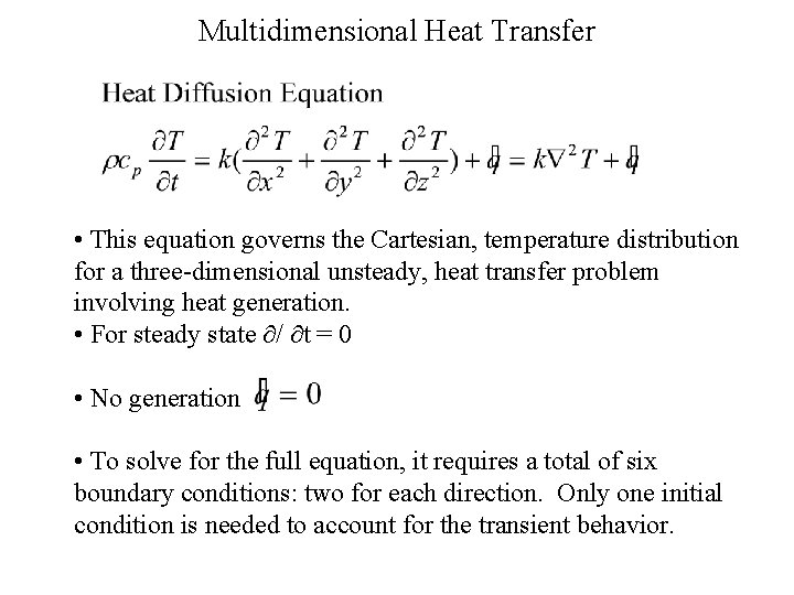
Multidimensional Heat Transfer • This equation governs the Cartesian, temperature distribution for a three-dimensional unsteady, heat transfer problem involving heat generation. • For steady state / t = 0 • No generation • To solve for the full equation, it requires a total of six boundary conditions: two for each direction. Only one initial condition is needed to account for the transient behavior.

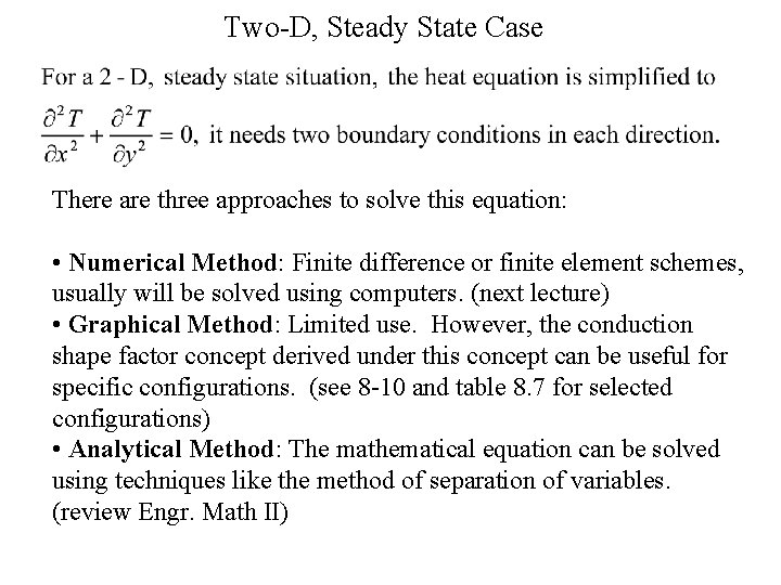
Two-D, Steady State Case There are three approaches to solve this equation: • Numerical Method: Finite difference or finite element schemes, usually will be solved using computers. (next lecture) • Graphical Method: Limited use. However, the conduction shape factor concept derived under this concept can be useful for specific configurations. (see 8 -10 and table 8. 7 for selected configurations) • Analytical Method: The mathematical equation can be solved using techniques like the method of separation of variables. (review Engr. Math II)

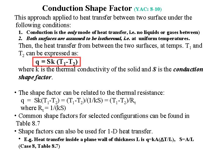
Conduction Shape Factor (YAC: 8 -10) This approach applied to heat transfer between two surface under the following conditions: 1. Conduction is the only mode of heat transfer, i. e. no liquids or gases between) 2. Both surfaces are assumed to be isothermal, i. e. at uniform temperatures. Then, the heat transfer from between the two surfaces, at temps. T 1 and T 2 can be expressed as: q = Sk (T 1 -T 2) where k is thermal conductivity of the solid and S is the conduction shape factor. • The shape factor can be related to thermal resistance: q = Sk(T 1 -T 2) = (T 1 -T 2)/(1/k. S) = (T 1 -T 2)/Rt where Rt = 1/(k. S) • Common shape factors for selected configurations can be found in Table 8. 7 • Shape factors can also be used for 1 -D heat transfer. • E. g. Heat transfer inside a plane wall of thickness L is q=k. A(DT/L), S=A/L (Case 8, Table 8. 7)

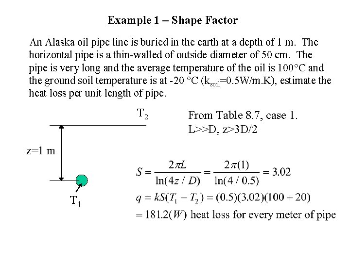
Example 1 – Shape Factor An Alaska oil pipe line is buried in the earth at a depth of 1 m. The horizontal pipe is a thin-walled of outside diameter of 50 cm. The pipe is very long and the average temperature of the oil is 100 C and the ground soil temperature is at -20 C (ksoil=0. 5 W/m. K), estimate the heat loss per unit length of pipe. T 2 z=1 m T 1 From Table 8. 7, case 1. L>>D, z>3 D/2

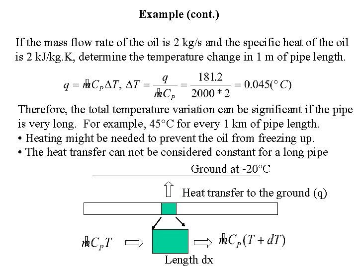
Example (cont. ) If the mass flow rate of the oil is 2 kg/s and the specific heat of the oil is 2 k. J/kg. K, determine the temperature change in 1 m of pipe length. Therefore, the total temperature variation can be significant if the pipe is very long. For example, 45 C for every 1 km of pipe length. • Heating might be needed to prevent the oil from freezing up. • The heat transfer can not be considered constant for a long pipe Ground at -20 C Heat transfer to the ground (q) Length dx

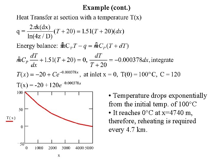
Example (cont. ) • Temperature drops exponentially from the initial temp. of 100 C • It reaches 0 C at x=4740 m, therefore, reheating is required every 4. 7 km.