MultiCriteria Analysis compromise programming Compromise programming CP Similar

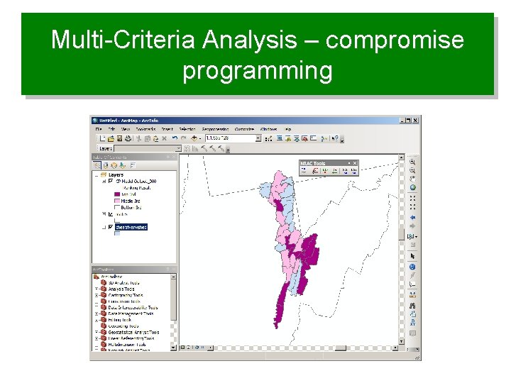
Multi-Criteria Analysis – compromise programming

Compromise programming (CP) • Similar to goal programming in that it uses the concept of minimum distance • A distance based technique that depends on the point of reference or “ideal” point • Attempts to minimize the “distance” from the ideal solution for a satisficing solution • The closest one to the ideal across all criteria is the compromise solution or compromise set

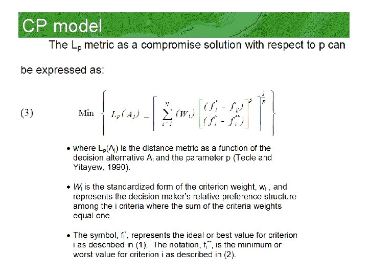
CP model

CP model notes • The larger the value of p, the greater the concern becomes. – For p = one, all weighted deviations are assumed to compensate each other perfectly. – For p = two, each weighted deviation is accounted for in direct proportion to its size. – As p approaches the limit of infinity, the alternative with the largest deviation completely dominates the distance measure (Zeleny, 1982).

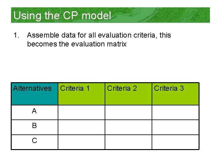
Using the CP model 1. Assemble data for all evaluation criteria, this becomes the evaluation matrix Alternatives A B C Criteria 1 Criteria 2 Criteria 3

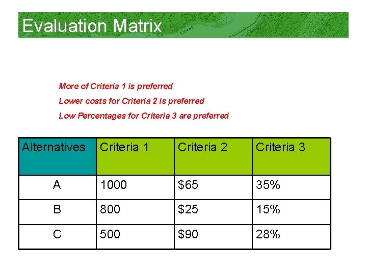
Evaluation Matrix More of Criteria 1 is preferred Lower costs for Criteria 2 is preferred Low Percentages for Criteria 3 are preferred Alternatives Criteria 1 Criteria 2 Criteria 3 A 1000 $65 35% B 800 $25 15% C 500 $90 28%

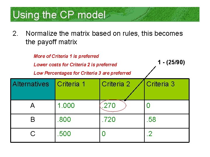
Using the CP model 2. Normalize the matrix based on rules, this becomes the payoff matrix More of Criteria 1 is preferred 1 - (25/90) Lower costs for Criteria 2 is preferred Low Percentages for Criteria 3 are preferred Alternatives Criteria 1 Criteria 2 Criteria 3 A 1. 000 . 270 0 B . 800 . 720 . 58 C . 500 0 . 2

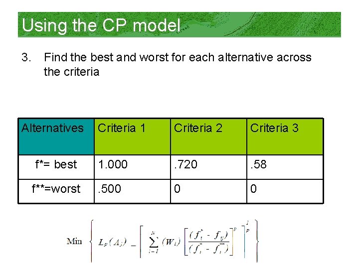
Using the CP model 3. Find the best and worst for each alternative across the criteria Alternatives Criteria 1 Criteria 2 Criteria 3 f*= best 1. 000 . 720 . 58 f**=worst . 500 0 0

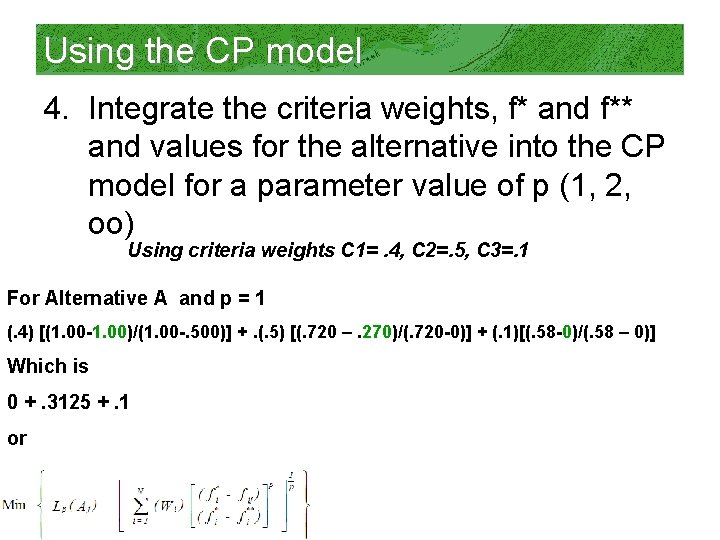
Using the CP model 4. Integrate the criteria weights, f* and f** and values for the alternative into the CP model for a parameter value of p (1, 2, oo) Using criteria weights C 1=. 4, C 2=. 5, C 3=. 1 For Alternative A and p = 1 (. 4) [(1. 00 -1. 00)/(1. 00 -. 500)] +. (. 5) [(. 720 –. 270)/(. 720 -0)] + (. 1)[(. 58 -0)/(. 58 – 0)] Which is 0 +. 3125 +. 1 or. 4125

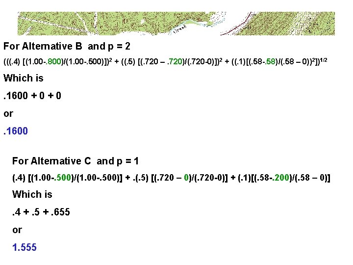
For Alternative B and p = 2 (((. 4) [(1. 00 -. 800)/(1. 00 -. 500)])2 + ((. 5) [(. 720 –. 720)/(. 720 -0)])2 + ((. 1)[(. 58 -. 58)/(. 58 – 0))2])1/2 Which is. 1600 + 0 or. 1600 For Alternative C and p = 1 (. 4) [(1. 00 -. 500)/(1. 00 -. 500)] +. (. 5) [(. 720 – 0)/(. 720 -0)] + (. 1)[(. 58 -. 200)/(. 58 – 0)] Which is. 4 +. 5 +. 655 or 1. 555

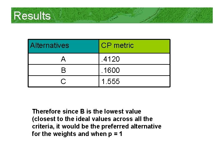
Results Alternatives A B C CP metric. 4120. 1600 1. 555 Therefore since B is the lowest value (closest to the ideal values across all the criteria, it would be the preferred alternative for the weights and when p = 1

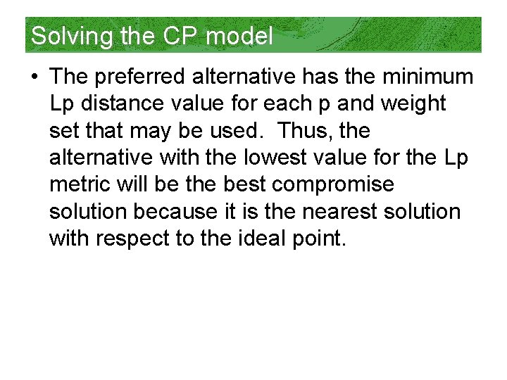
Solving the CP model • The preferred alternative has the minimum Lp distance value for each p and weight set that may be used. Thus, the alternative with the lowest value for the Lp metric will be the best compromise solution because it is the nearest solution with respect to the ideal point.

CP advantages • Simple conceptual structure • Simplicity makes it particularly useful for spatial decision problems in which decision makers tend to rely on their intuition and insight • The set of preferred compromise solutions can be ordered between the extreme criterion outcomes – (consequently, an implicit trade-off between criteria can be performed)

CP limitation • Except at the two extremes where p = 0 and p = oo there is no clear interpretation of the various values of the parameter p. • Therefore, use different weights or values for p to test overall robustness of results

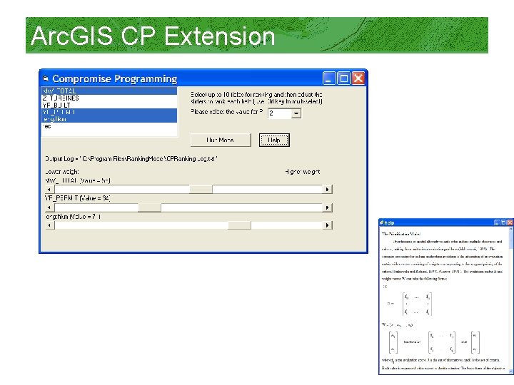
Arc. GIS CP Extension

Questions / Comments?