MSRI Program Mathematical Computational and Statistical Aspects of

MSRI Program: Mathematical, Computational and Statistical Aspects of Vision Learning and Inference in Low and Mid Level Vision Feb 21 -25, 2005 Is there a simple Statistical Model of Generic Natural Images? David Mumford

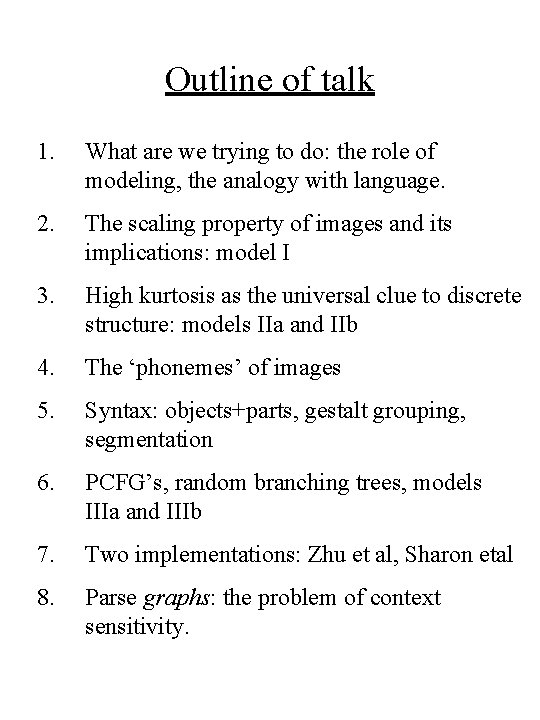
Outline of talk 1. What are we trying to do: the role of modeling, the analogy with language. 2. The scaling property of images and its implications: model I 3. High kurtosis as the universal clue to discrete structure: models IIa and IIb 4. The ‘phonemes’ of images 5. Syntax: objects+parts, gestalt grouping, segmentation 6. PCFG’s, random branching trees, models IIIa and IIIb 7. Two implementations: Zhu et al, Sharon etal 8. Parse graphs: the problem of context sensitivity.

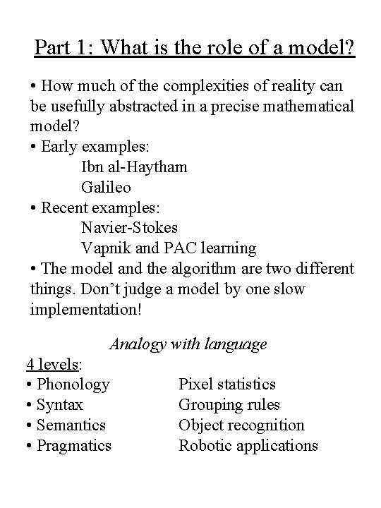
Part 1: What is the role of a model? • How much of the complexities of reality can be usefully abstracted in a precise mathematical model? • Early examples: Ibn al-Haytham Galileo • Recent examples: Navier-Stokes Vapnik and PAC learning • The model and the algorithm are two different things. Don’t judge a model by one slow implementation! Analogy with language 4 levels: • Phonology • Syntax • Semantics • Pragmatics Pixel statistics Grouping rules Object recognition Robotic applications

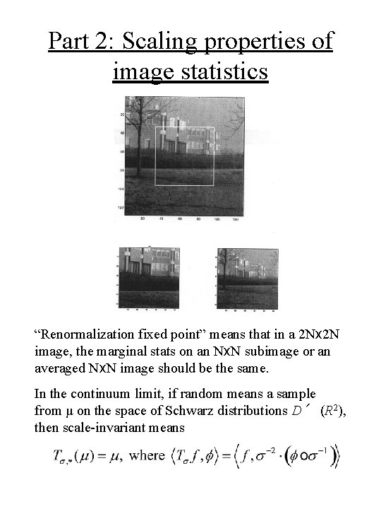
Part 2: Scaling properties of image statistics “Renormalization fixed point” means that in a 2 Nx 2 N image, the marginal stats on an Nx. N subimage or an averaged Nx. N image should be the same. In the continuum limit, if random means a sample from μ on the space of Schwarz distributions D′ (R 2), then scale-invariant means

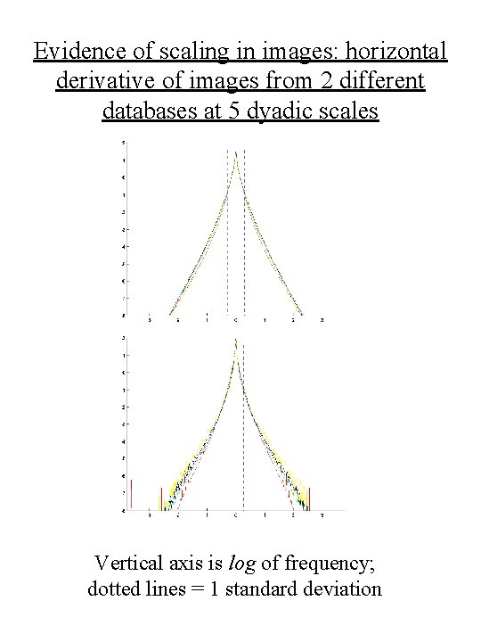
Evidence of scaling in images: horizontal derivative of images from 2 different databases at 5 dyadic scales Vertical axis is log of frequency; dotted lines = 1 standard deviation

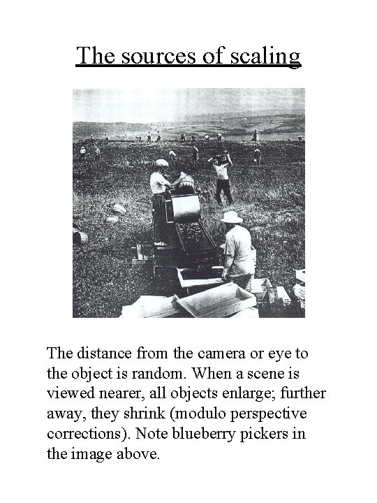
The sources of scaling The distance from the camera or eye to the object is random. When a scene is viewed nearer, all objects enlarge; further away, they shrink (modulo perspective corrections). Note blueberry pickers in the image above.

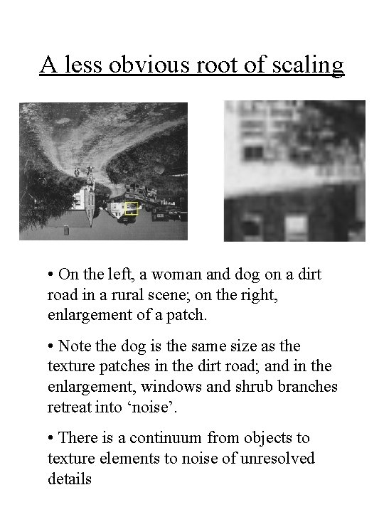
A less obvious root of scaling • On the left, a woman and dog on a dirt road in a rural scene; on the right, enlargement of a patch. • Note the dog is the same size as the texture patches in the dirt road; and in the enlargement, windows and shrub branches retreat into ‘noise’. • There is a continuum from objects to texture elements to noise of unresolved details

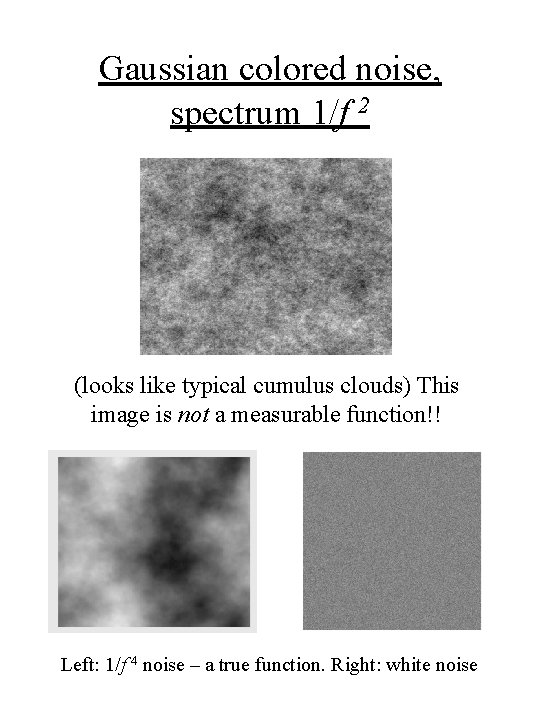
Gaussian colored noise, spectrum 1/f 2 (looks like typical cumulus clouds) This image is not a measurable function!! Left: 1/f 4 noise – a true function. Right: white noise

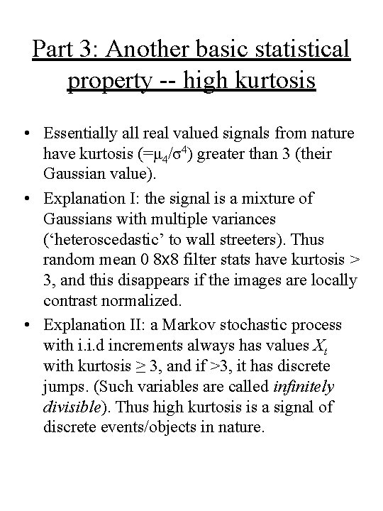
Part 3: Another basic statistical property -- high kurtosis • Essentially all real valued signals from nature have kurtosis (=μ 4/σ4) greater than 3 (their Gaussian value). • Explanation I: the signal is a mixture of Gaussians with multiple variances (‘heteroscedastic’ to wall streeters). Thus random mean 0 8 x 8 filter stats have kurtosis > 3, and this disappears if the images are locally contrast normalized. • Explanation II: a Markov stochastic process with i. i. d increments always has values Xt with kurtosis ≥ 3, and if >3, it has discrete jumps. (Such variables are called infinitely divisible). Thus high kurtosis is a signal of discrete events/objects in nature.

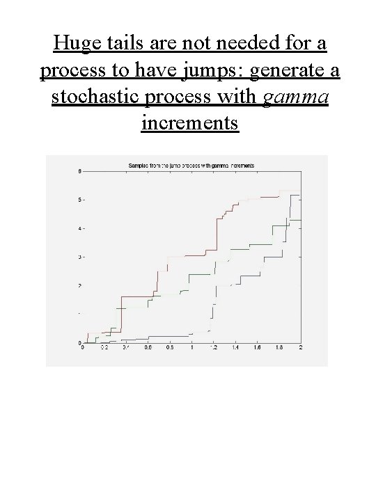
Huge tails are not needed for a process to have jumps: generate a stochastic process with gamma increments

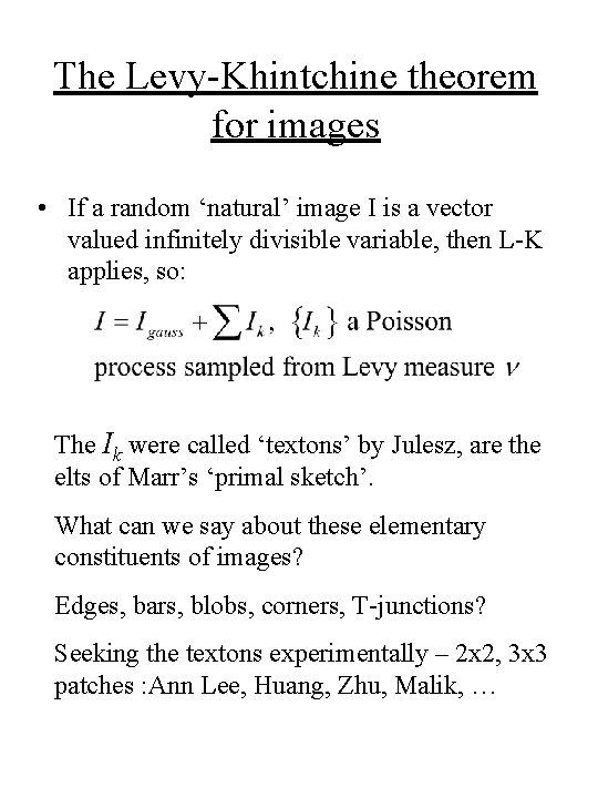
The Levy-Khintchine theorem for images • If a random ‘natural’ image I is a vector valued infinitely divisible variable, then L-K applies, so: The Ik were called ‘textons’ by Julesz, are the elts of Marr’s ‘primal sketch’. What can we say about these elementary constituents of images? Edges, bars, blobs, corners, T-junctions? Seeking the textons experimentally – 2 x 2, 3 x 3 patches : Ann Lee, Huang, Zhu, Malik, …

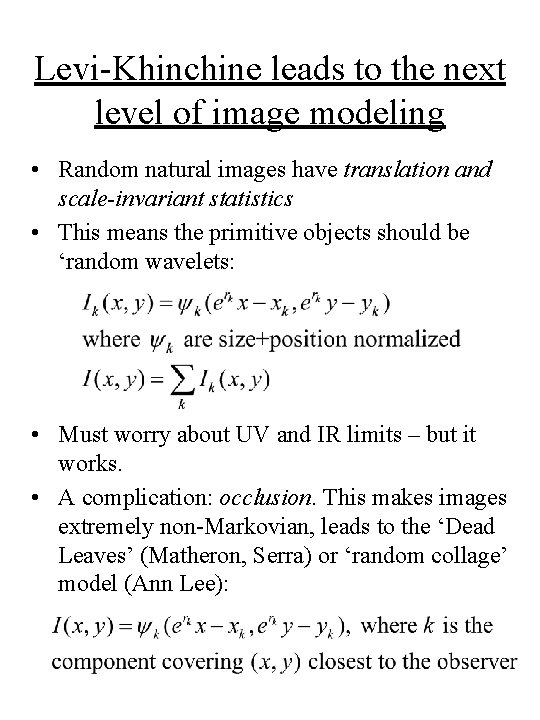
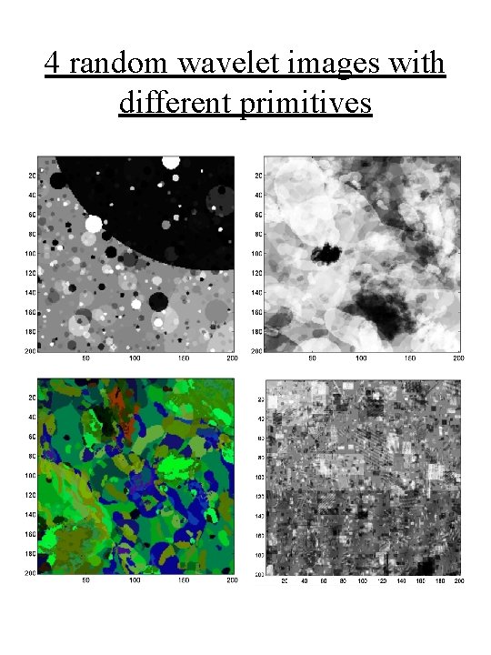
Levi-Khinchine leads to the next level of image modeling • Random natural images have translation and scale-invariant statistics • This means the primitive objects should be ‘random wavelets: • Must worry about UV and IR limits – but it works. • A complication: occlusion. This makes images extremely non-Markovian, leads to the ‘Dead Leaves’ (Matheron, Serra) or ‘random collage’ model (Ann Lee):

4 random wavelet images with different primitives

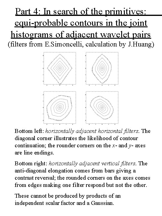
Part 4: In search of the primitives: equi-probable contours in the joint histograms of adjacent wavelet pairs (filters from E. Simoncelli, calculation by J. Huang) Bottom left: horizontally adjacent horizontal filters. The diagonal corner illustrates the likelihood of contour continuation; the rounder corners on the x- and y- axes are line endings. Bottom right: horizontally adjacent vertical filters. The anti-diagonal elongation comes from bars giving a contrast reversal; the rounded corners on the axes comes from edges making one filter respond but not the other. These cannot be produced by products of an independent scalar factor and a Gaussian.

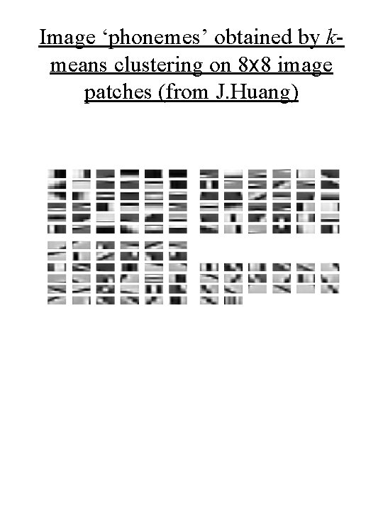
Image ‘phonemes’ obtained by kmeans clustering on 8 x 8 image patches (from J. Huang)

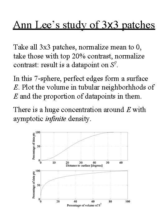
Ann Lee’s study of 3 x 3 patches Take all 3 x 3 patches, normalize mean to 0, take those with top 20% contrast, normalize contrast: result is a datapoint on S 7. In this 7 -sphere, perfect edges form a surface E. Plot the volume in tubular neighborhhods of E and the proportion of datapoints in them. There is a huge concentration around E with aymptotic infinite density.

Part 5. Grouping laws and the syntax of images • Our models are too homogeneous. Natural world scenes have more homogeneously colored/textured parts with discontinuities between them: this is segmentation. • Is segmentation well-defined? YES if you let it be hierarchical and not one fixed domain decomposition, allowing for the scaling of images.

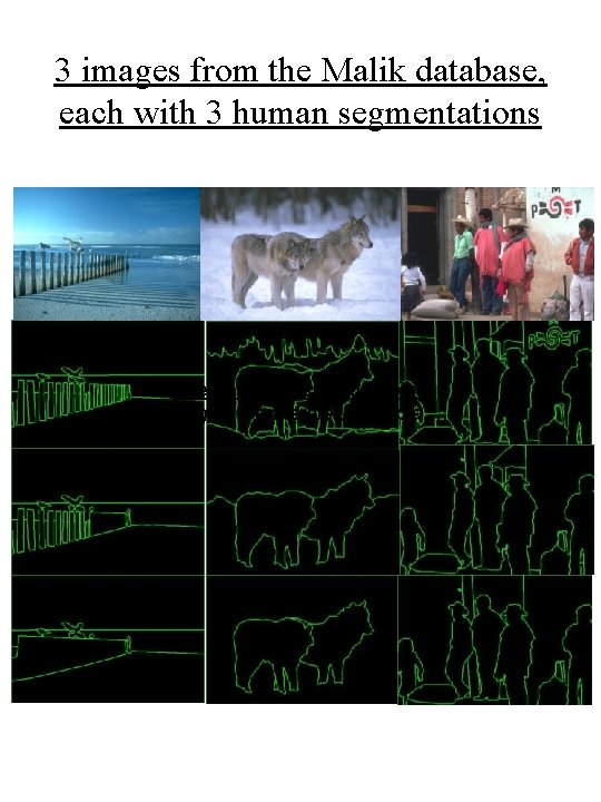
3 images from the Malik database, each with 3 human segmentations The gestalt rules of grouping (Metzger, Wertheimer, Kanisza, …)

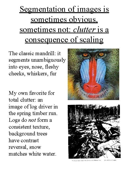
Segmentation of images is sometimes obvious, sometimes not: clutter is a consequence of scaling The classic mandrill: it segments unambiguously into eyes, nose, fleshy cheeks, whiskers, fur My own favorite for total clutter: an image of log driver in the spring timber run. Logs do not form a consistent texture, background trees have contrast reversal, snow matches white water.

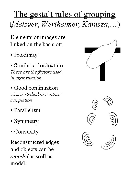
The gestalt rules of grouping (Metzger, Wertheimer, Kanisza, …) Elements of images are linked on the basis of: • Proximity • Similar color/texture These are the factors used in segmentation • Good continuation This is studied as contour completion • Parallelism • Symmetry • Convexity Reconstructed edges and objects can be amodal as well as modal:

Part 6: Random branching trees • Start at the root. Each node decides to have k children with probability pk, where Σ pk = 1. Continue infinietly or until no more children. • λ= Σ kpk is the expected # of children; if λ≤ 1, then the tree is a. s. finite; if λ>1, it is infinite with pos. prob. • Can put labels, from some finite set L, on the nodes and make a labelled tree from a prob. distr. which assigns probabilities to a label {l} having k children with labels {l 1, . . . , lk}. • This is identical to what linguists call PCFG’s (=probabilistic context-free grammars). For them, L is the set of attributed phrases (e. g. ‘singular feminine noun phrases’) plus the lexicon (which can have no children) and the tree is assumed a. s. to be finite.

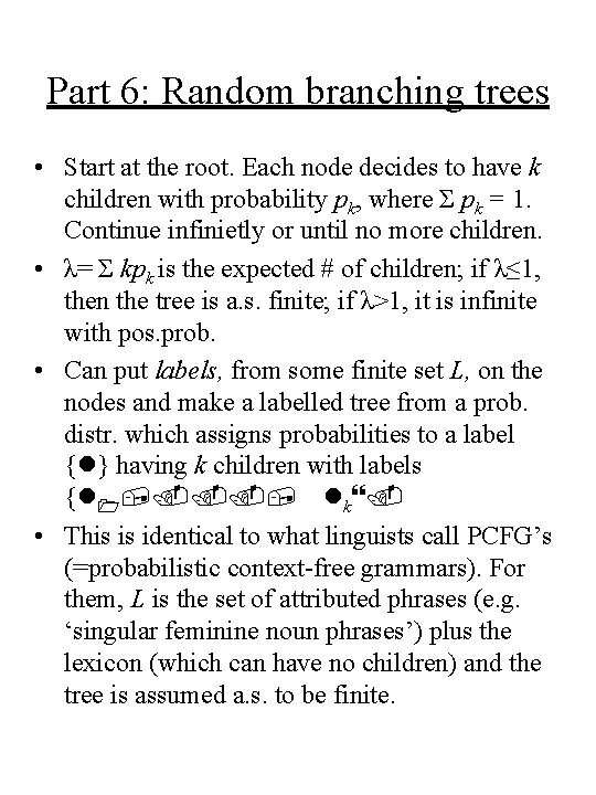
Graft random branching trees into the random wavelet model 1. Seed scale space with a Poisson process (xi, yi, ri) with density Cdxdydr/r 3. 2. Let each node grow a tree with growth rate <(r/r 0)2. 3. Put primitives on seeds, e. g. face, tree, road. It passes attributes to its children, e. g. eyes, trunk, car.

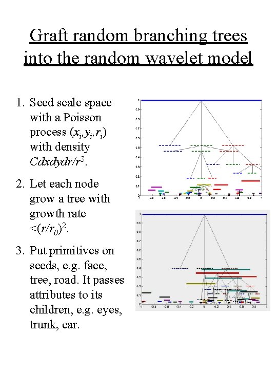
Part 7 a: Zhu’s algorithms: top-down synthesis and bottom up tree construction

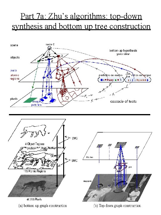
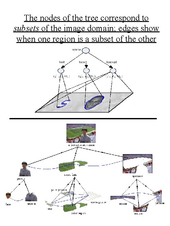
The nodes of the tree correspond to subsets of the image domain; edges show when one region is a subset of the other

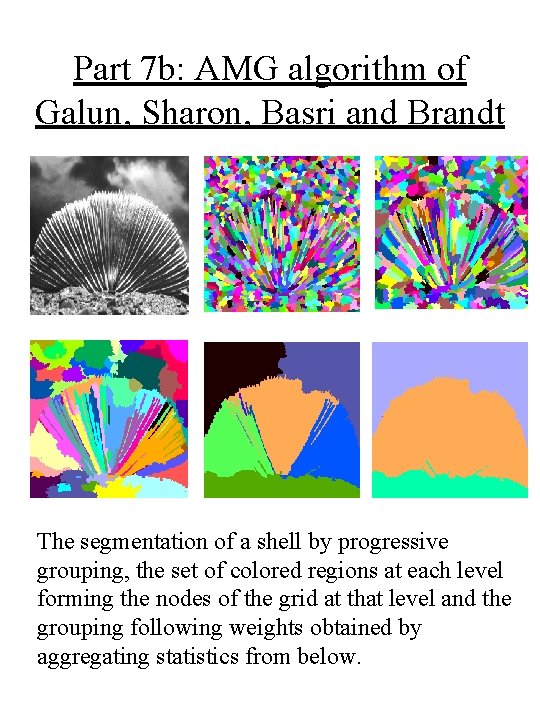
Part 7 b: AMG algorithm of Galun, Sharon, Basri and Brandt The segmentation of a shell by progressive grouping, the set of colored regions at each level forming the nodes of the grid at that level and the grouping following weights obtained by aggregating statistics from below.

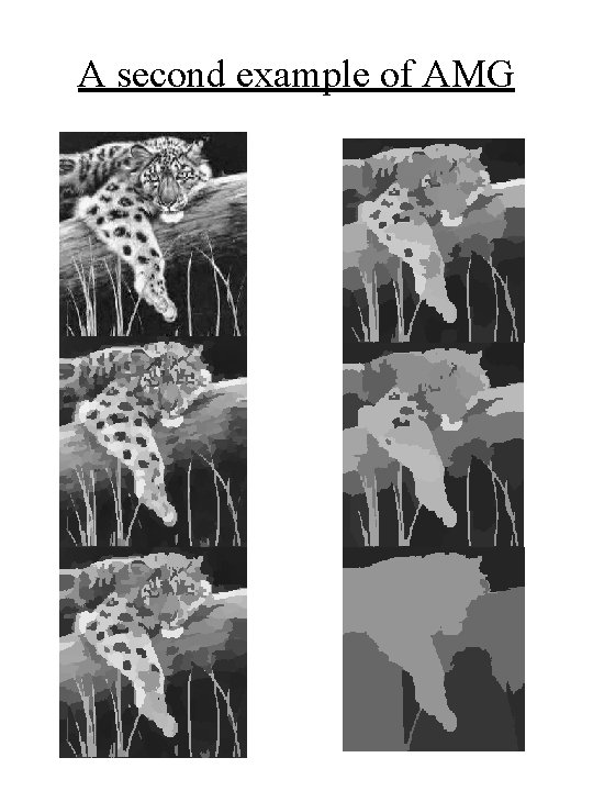
A second example of AMG

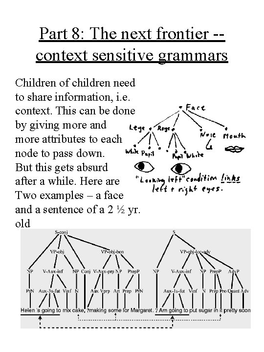
Part 8: The next frontier -context sensitive grammars Children of children need to share information, i. e. context. This can be done by giving more and more attributes to each node to pass down. But this gets absurd after a while. Here are Two examples – a face and a sentence of a 2 ½ yr. old

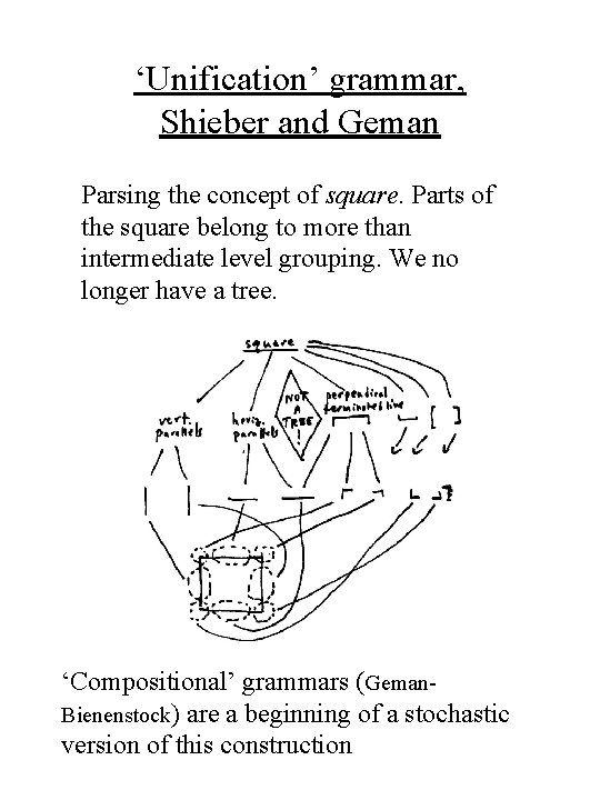
‘Unification’ grammar, Shieber and Geman Parsing the concept of square. Parts of the square belong to more than intermediate level grouping. We no longer have a tree. ‘Compositional’ grammars (Geman. Bienenstock) are a beginning of a stochastic version of this construction