MS 15 DataAware Parallel Computing DataDriven Parallelization in

MS 15: Data-Aware Parallel Computing • Data-Driven Parallelization in Multi-Scale Applications – Ashok Srinivasan, Florida State University • Dynamic Data Driven Finite Element Modeling of Brain Shape Deformation During Neurosurgery – Amitava Majumdar, San Diego Supercomputer Center • Dynamic Computations in Large-Scale Graphs – David Bader, Georgia Tech • Tackling Obesity in Children – Radha Nandkumar, NCSA www. cs. fsu. edu/~asriniva/presentations/siampp 06

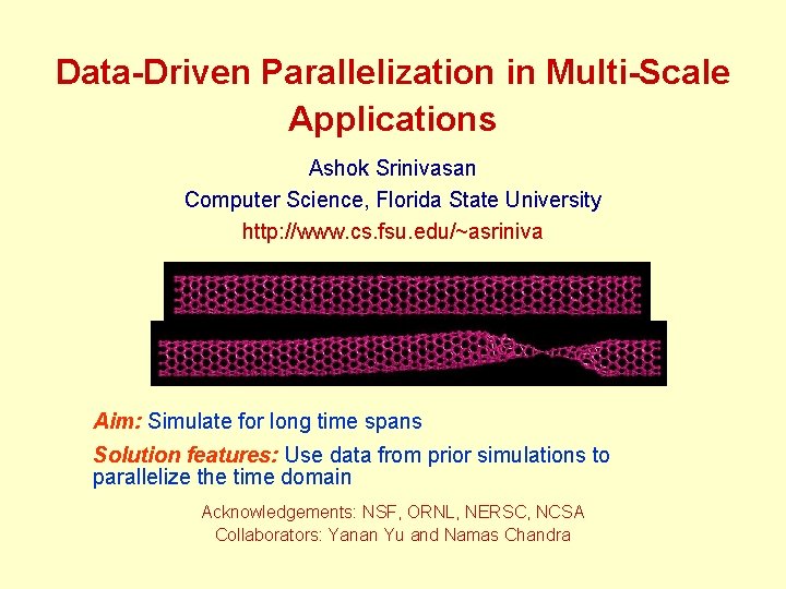
Data-Driven Parallelization in Multi-Scale Applications Ashok Srinivasan Computer Science, Florida State University http: //www. cs. fsu. edu/~asriniva Aim: Simulate for long time spans Solution features: Use data from prior simulations to parallelize the time domain Acknowledgements: NSF, ORNL, NERSC, NCSA Collaborators: Yanan Yu and Namas Chandra

Outline • Background – Limitations of Conventional Parallelization – Example Application: Carbon Nanotube Tensile Test • Small Time Step Size in Molecular Dynamics Simulations • Data-Driven Time Parallelization • Experimental Results – Scaled efficiently to ~ 1000 processors, for a problem where conventional parallelization scales to just 2 -3 processors • Other time parallelization approaches • Conclusions

Background • Limitations of Conventional Parallelization • Example Application: Carbon Nanotube Tensile Test – Molecular Dynamics Simulations • Problems with Multiple Time-Scales

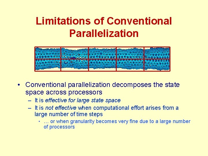
Limitations of Conventional Parallelization • Conventional parallelization decomposes the state space across processors – It is effective for large state space – It is not effective when computational effort arises from a large number of time steps • … or when granularity becomes very fine due to a large number of processors

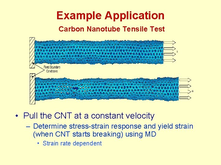
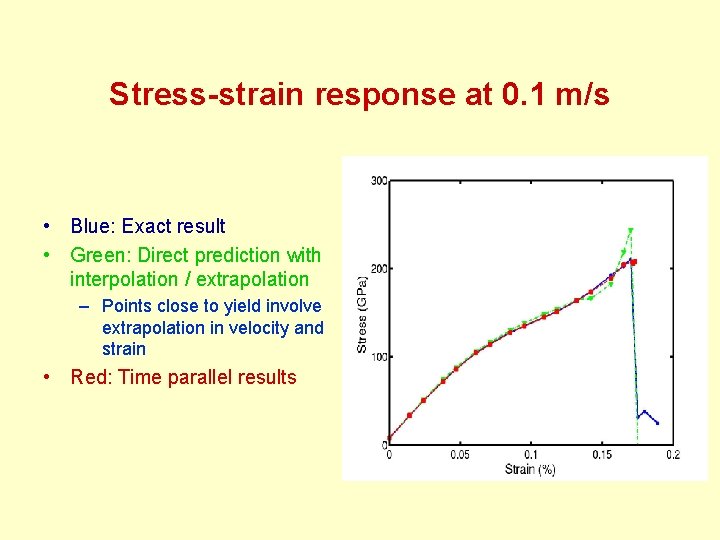
Example Application Carbon Nanotube Tensile Test • Pull the CNT at a constant velocity – Determine stress-strain response and yield strain (when CNT starts breaking) using MD • Strain rate dependent

A Drawback of Molecular Dynamics • Molecular dynamics – In each time step, forces of atoms on each other modeled using some potential – After force is computed, update positions – Repeat for desired number of time steps • Time steps size ~ 10 – 15 seconds, due to physical and numerical considerations – Desired time range is much larger • A million time steps are required to reach 10 -9 s • Around a day of computing for a 3000 -atom CNT • MD uses unrealistically large strain-rates

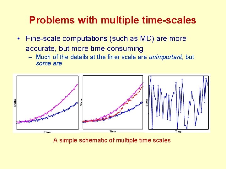
Problems with multiple time-scales • Fine-scale computations (such as MD) are more accurate, but more time consuming – Much of the details at the finer scale are unimportant, but some are A simple schematic of multiple time scales

Data-Driven Time Parallelization • Time parallelization • Data Driven Prediction – Dimensionality Reduction – Relate Simulation Parameters – Static Prediction – Dynamic Prediction • Verification

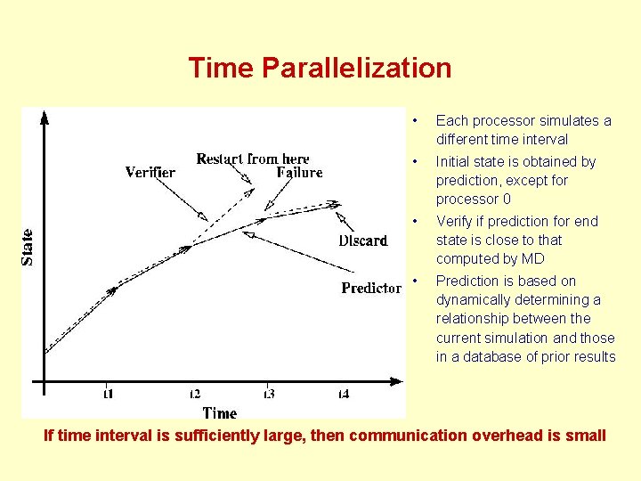
Time Parallelization • Each processor simulates a different time interval • Initial state is obtained by prediction, except for processor 0 • Verify if prediction for end state is close to that computed by MD • Prediction is based on dynamically determining a relationship between the current simulation and those in a database of prior results If time interval is sufficiently large, then communication overhead is small

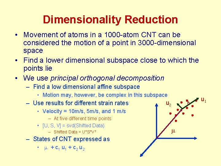
Dimensionality Reduction • Movement of atoms in a 1000 -atom CNT can be considered the motion of a point in 3000 -dimensional space • Find a lower dimensional subspace close to which the points lie • We use principal orthogonal decomposition – Find a low dimensional affine subspace • Motion may, however, be complex in this subspace – Use results for different strain rates u u • Velocity = 10 m/s, 5 m/s, and 1 m/s – At five different time points • [U, S, V] = svd(Shifted Data) – Shifted Data = U*S*VT – States of CNT expressed as • m + c 1 u 1 + c 2 u 2 m

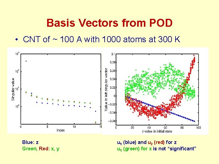
Basis Vectors from POD • CNT of ~ 100 A with 1000 atoms at 300 K Blue: z Green, Red: x, y u 1 (blue) and u 2 (red) for z u 1 (green) for x is not “significant”

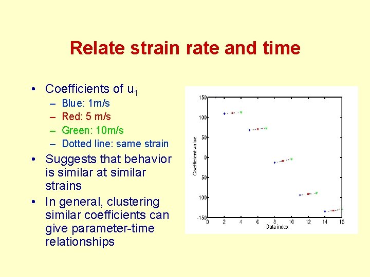
Relate strain rate and time • Coefficients of u 1 – – Blue: 1 m/s Red: 5 m/s Green: 10 m/s Dotted line: same strain • Suggests that behavior is similar at similar strains • In general, clustering similar coefficients can give parameter-time relationships

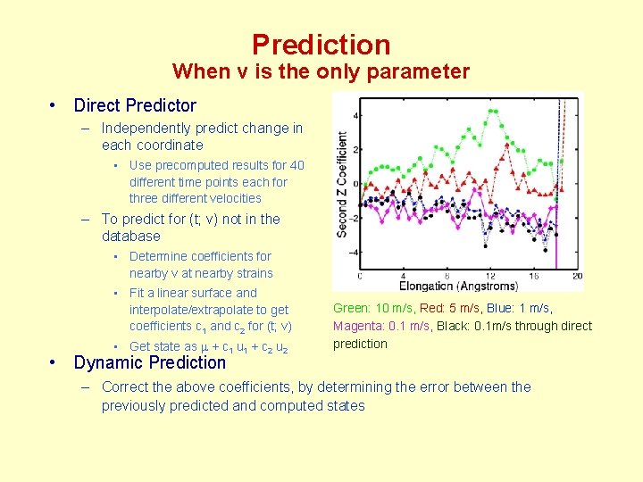
Prediction When v is the only parameter • Direct Predictor – Independently predict change in each coordinate • Use precomputed results for 40 different time points each for three different velocities – To predict for (t; v) not in the database • Determine coefficients for nearby v at nearby strains • Fit a linear surface and interpolate/extrapolate to get coefficients c 1 and c 2 for (t; v) • Get state as m + c 1 u 1 + c 2 u 2 Green: 10 m/s, Red: 5 m/s, Blue: 1 m/s, Magenta: 0. 1 m/s, Black: 0. 1 m/s through direct prediction • Dynamic Prediction – Correct the above coefficients, by determining the error between the previously predicted and computed states

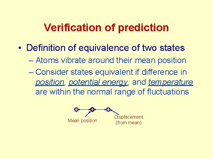
Verification of prediction • Definition of equivalence of two states – Atoms vibrate around their mean position – Consider states equivalent if difference in position, potential energy, and temperature are within the normal range of fluctuations Mean position Displacement (from mean)

Experimental Results • Relate simulations with different strain rates – Use the above strategy directly • Relate simulations with different strain rates and different CNT sizes – Express basis vectors in a different functional form • Relate simulations with different temperatures and strain rates – Dynamically identify different simulations that are similar in current behavior

Stress-strain response at 0. 1 m/s • Blue: Exact result • Green: Direct prediction with interpolation / extrapolation – Points close to yield involve extrapolation in velocity and strain • Red: Time parallel results

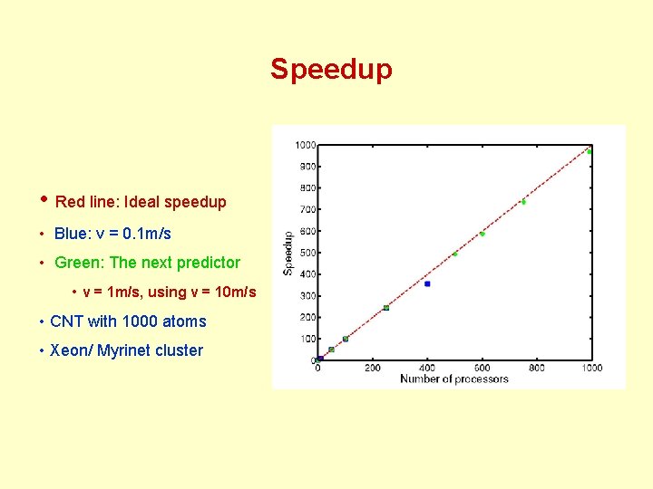
Speedup • Red line: Ideal speedup • Blue: v = 0. 1 m/s • Green: The next predictor • v = 1 m/s, using v = 10 m/s • CNT with 1000 atoms • Xeon/ Myrinet cluster

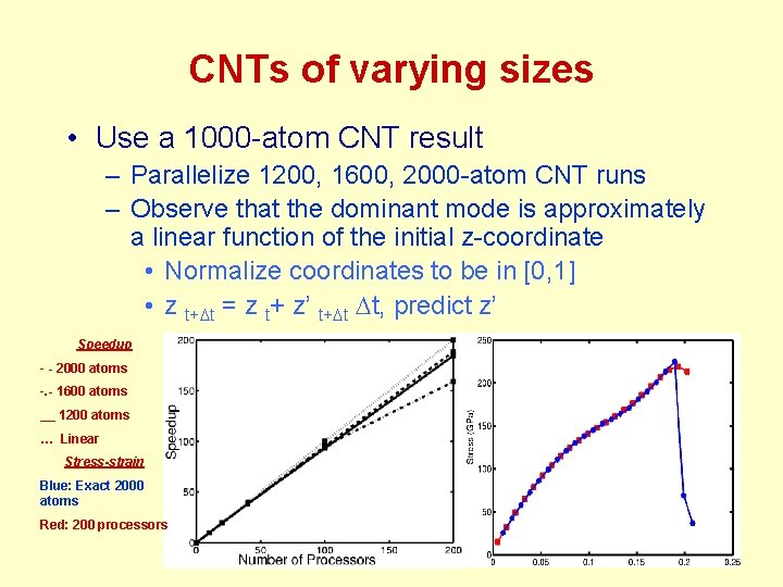
CNTs of varying sizes • Use a 1000 -atom CNT result – Parallelize 1200, 1600, 2000 -atom CNT runs – Observe that the dominant mode is approximately a linear function of the initial z-coordinate • Normalize coordinates to be in [0, 1] • z t+Dt = z t+ z’ t+Dt Dt, predict z’ Speedup - - 2000 atoms -. - 1600 atoms __ 1200 atoms … Linear Stress-strain Blue: Exact 2000 atoms Red: 200 processors

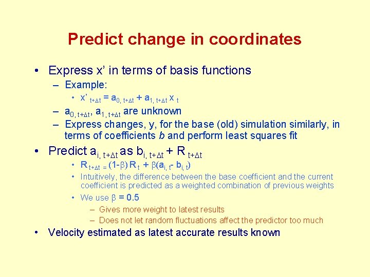
Predict change in coordinates • Express x’ in terms of basis functions – Example: • x’ t+Dt = a 0, t+Dt + a 1, t+Dt x t – a 0, t+Dt, a 1, t+Dt are unknown – Express changes, y, for the base (old) simulation similarly, in terms of coefficients b and perform least squares fit • Predict ai, t+Dt as bi, t+Dt + R t+Dt • R t+Dt = (1 -b) R t + b(ai, t- bi, t) • Intuitively, the difference between the base coefficient and the current coefficient is predicted as a weighted combination of previous weights • We use b = 0. 5 – Gives more weight to latest results – Does not let random fluctuations affect the predictor too much • Velocity estimated as latest accurate results known

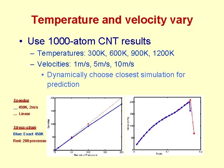
Temperature and velocity vary • Use 1000 -atom CNT results – Temperatures: 300 K, 600 K, 900 K, 1200 K – Velocities: 1 m/s, 5 m/s, 10 m/s • Dynamically choose closest simulation for prediction Speedup __ 450 K, 2 m/s … Linear Stress-strain Blue: Exact 450 K Red: 200 processors

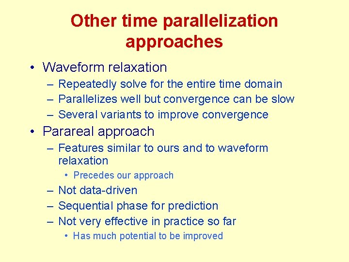
Other time parallelization approaches • Waveform relaxation – Repeatedly solve for the entire time domain – Parallelizes well but convergence can be slow – Several variants to improve convergence • Parareal approach – Features similar to ours and to waveform relaxation • Precedes our approach – Not data-driven – Sequential phase for prediction – Not very effective in practice so far • Has much potential to be improved

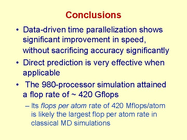
Conclusions • Data-driven time parallelization shows significant improvement in speed, without sacrificing accuracy significantly • Direct prediction is very effective when applicable • The 980 -processor simulation attained a flop rate of ~ 420 Gflops – Its flops per atom rate of 420 Mflops/atom is likely the largest flop per atom rate in classical MD simulations

Future Work • More complex problems – Better prediction • POD is good for representing data, but not necessarily for identifying patterns • Use better dimensionality reduction / reduced order modeling techniques • Use experimental data for prediction – Better learning – Better verification – In CP 8: Application of Dimensionality Reduction Techniques to Time Parallelization, Yanan Yu • Tomorrow, 2: 30 – 3: 00 pm