MOVING AVERAGES AND EXPONENTIAL SMOOTHING Introduction Forecasting methods

MOVING AVERAGES AND EXPONENTIAL SMOOTHING

Introduction • Forecasting methods: – Averaging methods. • Equally weighted observations – Exponential Smoothing methods. • Unequal set of weights to past data, where the weights decay exponentially from the most recent to the most distant data points. • These parameters (with values between 0 and 1) will determine the unequal weights to be applied to past data.

Introduction • Averaging methods – If a time series is generated by a constant process subject to random error, then mean is a useful statistic and can be used as a forecast for the next period. – Averaging methods are suitable for stationary time series data where the series is in equilibrium around a constant value ( the underlying mean) with a constant variance over time.

Introduction • Exponential smoothing methods – The simplest exponential smoothing method is the single smoothing (SES) method where only one parameter needs to be estimated – Holt’s method makes use of two different parameters and allows forecasting for series with trend. – Holt-Winters’ method involves three smoothing parameters to smooth the data, the trend and the seasonal index.

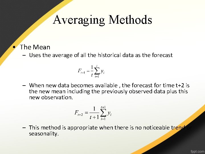
Averaging Methods • The Mean – Uses the average of all the historical data as the forecast – When new data becomes available , the forecast for time t+2 is the new mean including the previously observed data plus this new observation. – This method is appropriate when there is no noticeable trend or seasonality.

Averaging Methods • The moving average for time period t is the mean of the k most recent observations. • The constant number k is specified at the outset. • The smaller the number k, the more weight is given to recent periods. • The greater the number k, the less weight is given to more recent periods.

Single Moving Averages • A large k is desirable when there are wide, infrequent fluctuations in the series. • A small k is most desirable when there are sudden shifts in the level of series. • For quarterly data, a four-quarter moving average, MA(4), eliminates or averages out seasonal effects.

Single Moving Averages • For monthly data, a 12 -month moving average, MA(12), eliminate or averages out seasonal effect. • Equal weights are assigned to each observation used in the average. • Each new data point is included in the average as it becomes available, and the oldest data point is discarded.

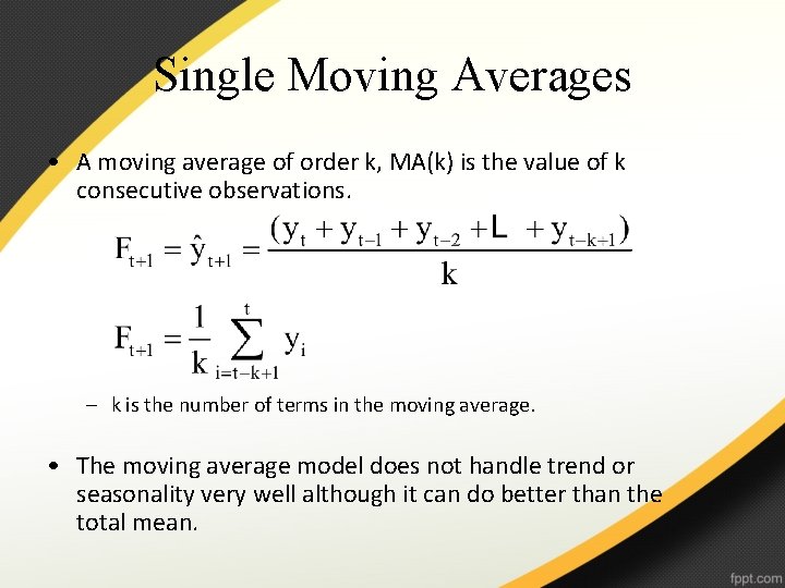
Single Moving Averages • A moving average of order k, MA(k) is the value of k consecutive observations. – k is the number of terms in the moving average. • The moving average model does not handle trend or seasonality very well although it can do better than the total mean.

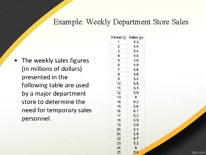
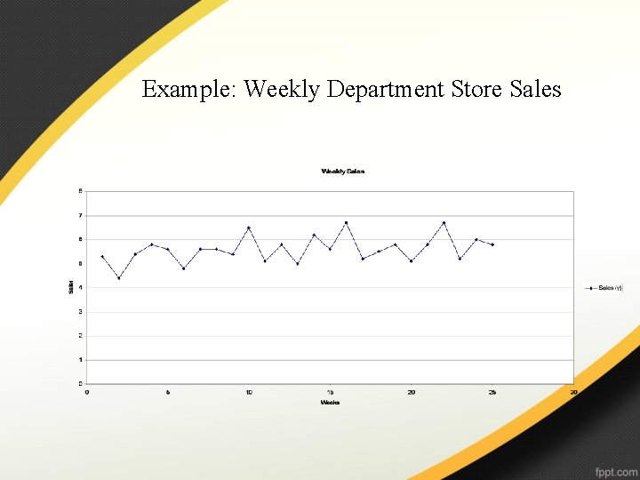
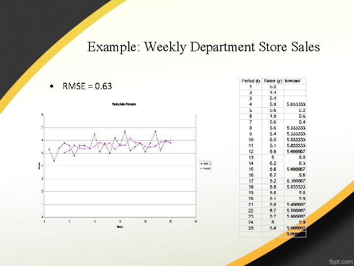
Example: Weekly Department Store Sales • The weekly sales figures (in millions of dollars) presented in the following table are used by a major department store to determine the need for temporary sales personnel.

Example: Weekly Department Store Sales

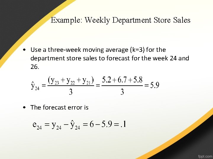
Example: Weekly Department Store Sales • Use a three-week moving average (k=3) for the department store sales to forecast for the week 24 and 26. • The forecast error is

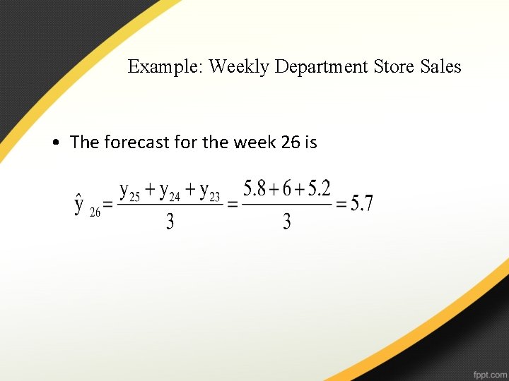
Example: Weekly Department Store Sales • The forecast for the week 26 is

Example: Weekly Department Store Sales • RMSE = 0. 63

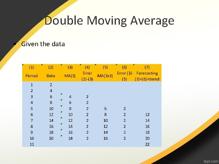
Double Moving Average • Given the data

Double Moving Average • Forecasting procedure: – Usingle moving average at time t (St’) – Fitting: the difference between single moving average and double moving average at time t (St’ – St’’) – Fitting: trend from t period to t+1 period (or to t+m period if we want to forecast m period)

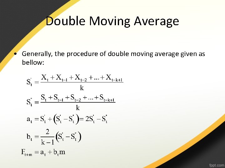
Double Moving Average • Generally, the procedure of double moving average given as bellow: